Examples using Transfer Functions

Proportional–Integral–Derivative (PID) control

A PID controller is one of the most widely used feedback control laws. It computes the control input based on the error signal

\[ e(t) = r(t) - y(t), \]

where \(r(t)\) is the reference input and \(y(t)\) is the system output.

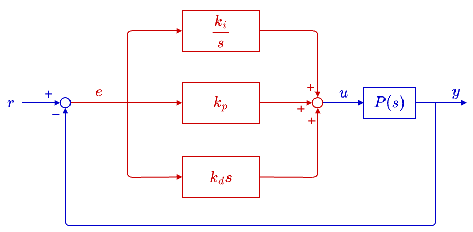
A PID controller generates the control input \(u(t)\) as a combination of three terms:

\[ u(t) = k_p e(t) + k_i \int_0^t e(\tau)\, d\tau + k_d \frac{de(t)}{dt}. \]

Each term plays a distinct role:

Proportional (P) \(\left(k_p e(t)\right)\): Reacts to the current error.

Integral (I) \(\left(t_0^t e(\tau)\, d\tau\right)\): Accumulates past error, eliminating steady-state offset.

Derivative (D) \(\left(k_d \frac{de(t)}{dt}\right)\): Anticipates future error by responding to its rate of change.

The transfer function for the controller from \(e\) to \(u\) is

\[ C(s) = k_p + \frac{k_i}{s} + k_d s. \]

Let the plant to be controlled have the transfer function \(P(s)\) (as shown in the digram above).

Steady-state reference tracking

We will now analyze the effect of PID controllers on stead-state reference tracking.

The closed-loop transfer function from \(r\) to \(y\) is

\[ G_{ry}(s) = \frac{P(s)C(s)}{1 + P(s)C(s)}. \]

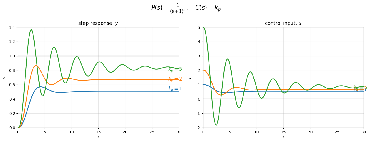
(Only) Proportional control

First, consider pure proportional feedback, i.e., \(k_i = 0\) and \(k_d = 0.\)

For a unit step reference input, the steady-state output is

\[ y_{ss} = G_{ry}(0) = \frac{C(0)P(0)}{1 + C(0)P(0)}. \]

Since $\( C(s) = k_p \;\;\Rightarrow\;\; C(0) = k_p, \)$

we obtain

\[ y_{ss} = \frac{k_p P(0)}{1 + k_p P(0)}. \]

Key observations: Proportional control alone cannot eliminate steady-state error, but it can reduce it.

• Increasing \(k_p\) makes \(y_{ss}\) closer to 1.

• However, \(y_{ss} \neq 1\) for any finite \(k_p\).

From the example below, increasing \(k_p\):

• Reduces the steady-state error.

• But also introduces (larger) oscillations and increases overshoot.

Steady-state reference tracking (continued)

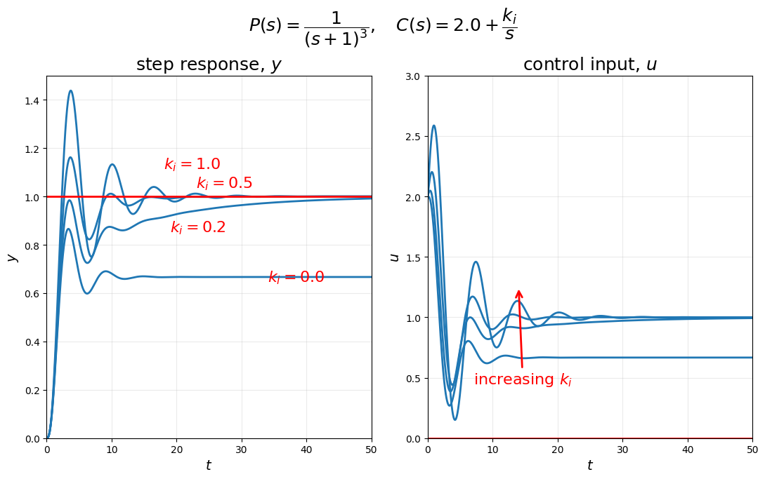
Proportional–Integral (PI) control

Introduce integral feedback: $\( C(s) = k_p + \frac{k_i}{s}. \)$

The closed-loop transfer function from \(r\) to \(y\) is $\( G_{ry}(s) = \frac{\left(k_p + \frac{k_i}{s}\right) P(s)}{1 + \left(k_p + \frac{k_i}{s}\right) P(s)}= \frac{(k_p s + k_i) P(s)}{s + (k_p s + k_i) P(s)}. \)$

For a unit step reference input, $\( G_{ry}(0) = \frac{k_i P(0)}{k_i P(0)} = 1. \)$

Key observations:

• Perfect reference tracking (zero steady-state error) is achieved as long as \(k_i \neq 0\) (and the closed-loop system stays stable).

• This result is independent of the plant gain \(P(0)\); hence, it is robust to model uncertainty.

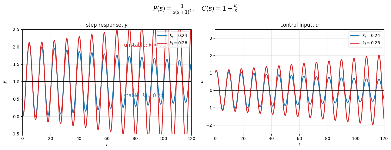
Based on the example below, increasing \(k_i\) increases the speed of the approach to the steady-state output. But, the system becomes more oscillatory, and may cease to be stable.

Steady-state reference tracking (continued)

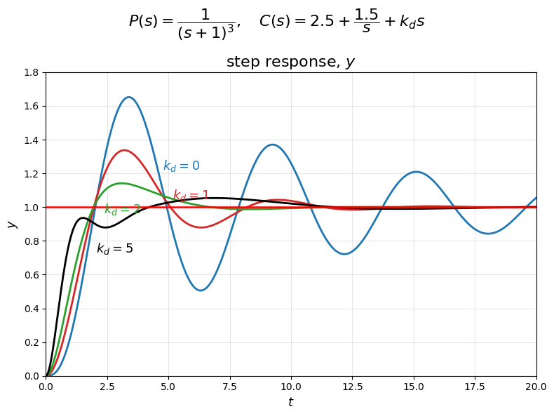
Proportional-integtral-derivative control

Let us now add the derivative term:

\[ C(s) = k_p + \frac{k_i}{s} + k_d s. \]

From the numerical example (with fixed \(k_p = 2.5\) and \(k_i = 1.5,\) as \(k_d\) increases, the closed-loop system becomes more damped. So, the derivative term increases damping and can improve transient behavior.

Let’s look at an example. Consider a second-order plant

\[ P(s) = \frac{1}{s^2 + \alpha_1 s + \alpha_2}. \]

We analyze the closed-loop behavior under derivative control only, with

\[ C(s) = k_d s. \]

The closed-loop transfer function is

\[ G_{ry}(s) = \frac{C(s)P(s)}{1 + C(s)P(s)} = \frac{k_d s}{s^2 + \alpha_1 s + \alpha_2 + k_d s}. \]

Thus, the closed-loop characteristic polynomial

\[ s^2 + (\alpha_1 + k_d)s + \alpha_2. \]

Comparing with a standard second-order system

\[ s^2 + 2\zeta \omega_n s + \omega_n^2, \]

we identify:

\[ 2\zeta \omega_n = \alpha_1 + k_d, \qquad \omega_n^2 = \alpha_2. \]

In conclusion, \(\alpha_2\) is unchanged; hence, the natural frequency \(\omega_n\) is unchanged. On the other hand, \(\alpha_1\) increases to \(\alpha_1 + k_d\); hence, the damping ratio \(\zeta\) increases.

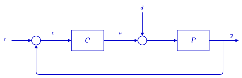
Another useful role of integral action: disturbance rejection

Consider the feedback system with an additive disturbance \(d\) entering at the plant input.

We now study integral action for disturbance attenuation, rather than reference tracking.

Assume \(r=0,\) and let \(d\) be a unit step disturbance.

Take a pure integral controller:

\[ C(s)=\frac{k_i}{s}. \]

The transfer function from \(d\) to \(y\) is

\[ G_{dy}(s)=\frac{P(s)}{1+P(s)C(s)}. \]

Substituting \(C(s)=\frac{k_i}{s}\) gives

\[ G_{dy}(s)=\frac{P(s)}{1+P(s)\frac{k_i}{s}} = \frac{sP(s)}{s+k_iP(s)}. \]

For a stable closed-loop system, the steady-state gain from a step disturbance is \(G_{dy}(0)\). Hence

\[ G_{dy}(0)=\frac{0}{k_i P(0)}=0. \]

Therefore, the steady-state output due to a unit step disturbance is zero.

Example: Comparing different PID controllers

Consider the feedback interconnection

and four differnt controllers: $\( \begin{aligned} C_1(s) &= 1, \\ C_2(s) &= 2, \\ C_3(s) &= 1 + \frac{1}{s}, \\ C_4(s) &= 1 + \frac{1}{s} + s. \end{aligned} \)$

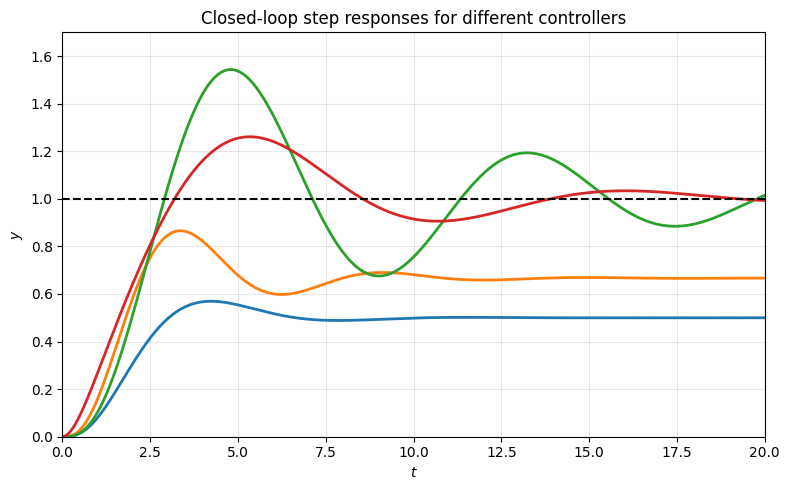
The figure below shows the unit step responses (shown in different colors) from \(r\) to \(y\) for the closed-loop system with these four different controllers. Match \(C_1, \ldots, C_4\) to the shown step responses.

• Blue: \(C_1(s)=1\): proportional control with smaller (than \(C_2\)) gain
  \(\Rightarrow\) slower response, larger steady-state error

• Orange: \(C_2(s)=2\): higher proportional gain
  \(\Rightarrow\) faster response, smaller steady-state error, more oscillation

• Green: \(C_3(s)=1+\frac{1}{s}\) (PI):
  \(\Rightarrow\) zero steady-state error, moderate oscillations

• Red: \(C_4(s)=1+\frac{1}{s}+s\) (PID):
  \(\Rightarrow\) zero steady-state error with improved damping

Example: Using the steady-state gain to determine an unknown parameter

Let the transfer function of a stable linear system be $\( G(s)=\frac{5}{s^2+3.2s+a}, \)\( where \)a$ is an unknown parameter.

Suppose the input is a constant step of amplitude \(2\), that is,

\[ u(t)=2, \qquad t\ge 0, \]

and the corresponding steady-state output is

\[ y_{ss}=4. \]

We want to determine the value of \(a\).

For a stable system, the steady-state gain under a step input is

\[ G(0). \]

Here,

\[ G(0)=\frac{5}{a}. \]

Since the input magnitude is \(2\) and the steady-state output is \(4\), the gain from input to output is

\[ \frac{4}{2}=2. \]

Therefore,

\[ G(0)=2. \]

Set

\[ \frac{5}{a}=2. \]

Hence,

\[ a=\frac{5}{2}=2.5. \]

Example: Determining the parameters of a second-order system from steady-state responses

Consider the stable second-order system

\[ \ddot y(t) + \alpha_1 \dot y(t) + \alpha_2 y(t) = u(t), \]

where \(\alpha_1\) and \(\alpha_2\) are unknown.

The corresponding transfer function from \(u\) to \(y\) is

\[ G(s) = \frac{1}{s^2 + \alpha_1 s + \alpha_2}. \]

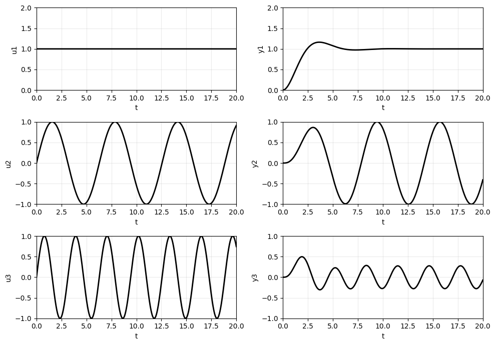
We use the input-output plots (shown below) to determine \(\alpha_1\) and \(\alpha_2\).

For the first input,

\[ u_1(t)=1. \]

From the plot, the steady-state output is

\[ y_{ss,1}(t) = 1. \]

For a stable system, the steady-state gain is

\[ G(0)=\frac{1}{\alpha_2}. \]

Since the input amplitude is \(1\) and the steady-state output is also \(1\), we get

\[ G(0)=1. \]

Hence

\[ \frac{1}{\alpha_2}=1 \quad\Rightarrow\quad \alpha_2=1. \]

Now consider a sinusoidal input with frequency \(\omega=1\).

The frequency response is

\[ G(j\omega)=\frac{1}{(j\omega)^2+\alpha_1 j\omega+\alpha_2}. \]

At \(\omega=1\), using \(\alpha_2=1\),

\[ G(j)=\frac{1}{-1+\alpha_1 j+1} =\frac{1}{\alpha_1 j}. \]

Therefore,

\[ |G(j)|=\frac{1}{\alpha_1}. \]

From the plot, the steady-state amplitude of \(y_2\) is approximately \(1\), while the input amplitude is also \(1\). Thus

\[ |G(j)|=1. \]

So

\[ \frac{1}{\alpha_1}=1 \quad\Rightarrow\quad \alpha_1=1. \]

Check with the third input (though it is not necessary to determine \(\alpha_1\) and \(\alpha_2\)). For

\[ u_3(t)=\sin(2t), \]

the predicted steady-state gain is

\[ |G(2j)|=\frac{1}{\sqrt{(1-2^2)^2 + (2\alpha_1)^2}} =\frac{1}{\sqrt{(1-4)^2 + 2^2}} =\frac{1}{\sqrt{13}} \approx 0.277. \]

This is consistent with the smaller amplitude seen in the plot for \(y_3\).

Exercise

Consider a plant \(P\) with transfer function

\[ P(s) = \frac{s}{s - 1}. \]

(a) Is the plant stable?

(b) Consider a controller, \(C\), with transfer function $\( C(s) = \frac{b}{s + c}. \)$

For the feedback loop consisting of \(P\) and \(C\) (with the usual negative \(( - )\) feedback convention), what is the closed-loop characteristic polynomial?

(c) Pick \(b\) and \(c\) (i.e., parameters of the control law) so that the roots of the closed-loop characteristic equation are $\( -1 \pm j. \)$