All rights reserved. For enrolled students only. Redistribution prohibited.

State Feedback Design

• State feedback control

• Controllable canonical form

• State feedback with feedforward control

• State feedback with integral action

How to scale up feedback control design?

The control design examples so far, we dealt with systems with small number states and with controllers were simple enough that we could carry out the design by hand. This approach won’t scale with the number of states. This naturally leads to a broader question:

How can we generalize these design ideas beyond specific examples?

We now introduce state feedback control design as a systematic approach that extends these ideas to general linear systems.

State feedback provides a way to shape the behavior of the closed-loop dynamics by systematically placing the poles, i.e., the eigenvalues of the closed-loop system matrix, or equivalently, the roots of its characteristic polynomial.

The setup

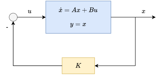
Linear system:

\[\dot{x} = Ax + Bu \quad \text{(with } x \in \mathbb{R}^n, u \in \mathbb{R}\text{)}\]

Controller:

\[u = -Kx \quad \text{(with } K \in \mathbb{R}^{1 \times n}\text{)}\]

It is important to note that the control signal is a function of the entire state \(x\) (hence, “state” feedback).

Let us know apply the design steps we practiced to this linear system and controller.

1. Determine the closed-loop dynamics:

   \[\dot{x} = Ax + Bu = Ax - BKx = (A - BK)x\]

   where \(A_{cl} = A - BK\).

2. Compute the characteristic polynomial of \(A - BK\):

   \[p(s) = \det(sI - (A - BK))\]

3. Pick \(K\) such that \(p(s)\) is equal to some given, desired polynomial \(p_{\text{des}}(s)\)

Two questions remain:

• How to pick K?

• How to identify \(p_{des}(s)\)?

We will begin with the latter.

How to identify a desired characteristic polynomial?

Earlier, we saw that the eigenvalues of the closed-loop system matrix \(A_{\mathrm{cl}}\), or equivalently, the roots of its characteristic polynomial—are directly related to stability and performance specifications.

In state-feedback design, it is therefore natural to begin by specifying a set of desired closed-loop eigenvalues, and then construct the corresponding desired characteristic polynomial.

Suppose we are given a set of desired closed-loop eigenvalues

\[ \lambda_1, \lambda_2, \dots, \lambda_n. \]

The desired characteristic polynomial is obtained by forming

\[ p_{\mathrm{des}}(s) = \prod_{i=1}^n (s - \lambda_i). \]

If the desired eigenvalues include complex numbers, they must appear in complex conjugate pairs so that the resulting polynomial has real coefficients.

Expanding this product yields a polynomial of the form

\[ p_{\mathrm{des}}(s) = s^n + a_{n-1}s^{n-1} + \cdots + a_1 s + a_0, \]

whose coefficients encode the design choice.

This polynomial is the target characteristic polynomial for the closed-loop system.

Example: Suppose we want the eigenvalues of \(A_{\mathrm{cl}}\) to be

\[ -1 + j,\quad -1 - j,\quad -10. \]

The desired characteristic polynomial is

\[\begin{split} \begin{aligned} p_{\mathrm{des}}(s) &= (s - (-1 + j))(s - (-1 - j))(s - (-10)) \\ &= (s + 1 - j)(s + 1 + j)(s + 10). \end{aligned} \end{split}\]

Multiplying the complex conjugate pair first,

\[ (s + 1 - j)(s + 1 + j) = (s + 1)^2 + 1 = s^2 + 2s + 2, \]

and then multiplying by (s + 10), we obtain

\[ p_{\mathrm{des}}(s) = (s^2 + 2s + 2)(s + 10) = s^3 + 12s^2 + 22s + 20. \]

What does \(\det(sI - (A - BK))\) look like?

To gain intiution to answer the first question “how to pick K,” let us consider another question first: How does the characteristic polynomial \(\det(sI - (A - BK))\) depend on the entries of \(K\)?

A small case illustrates the key difficulty. Consider a \(2\times 2\) system with

\[\begin{split} A=\begin{bmatrix}a_{11}&a_{12}\\ a_{21}&a_{22}\end{bmatrix},\quad B=\begin{bmatrix}b_1\\ b_2\end{bmatrix},\quad K=\begin{bmatrix}k_1&k_2\end{bmatrix}. \end{split}\]

Then

\[\begin{split} A - BK = \begin{bmatrix} a_{11}-b_1k_1 & a_{12}-b_1k_2\\ a_{21}-b_2k_1 & a_{22}-b_2k_2 \end{bmatrix}. \end{split}\]

The characteristic polynomial is

\[\begin{split} p_{\mathrm{cl}}(s) = \det\!\begin{bmatrix} s-(a_{11}-b_1k_1) & -(a_{12}-b_1k_2)\\ -(a_{21}-b_2k_1) & s-(a_{22}-b_2k_2) \end{bmatrix}. \end{split}\]

Expanding this determinant yields a quadratic polynomial in \(s\), whose coefficients depend on \(k_1\) and \(k_2\) in a nontrivial way through products and sums of the entries of \(A\), \(B\), and \(K\).

Even in this simple \(2\times 2\) case, the relationship between the entries of \(K\) and the coefficients of \(p_{\mathrm{cl}}(s)\) is already coupled and indirect.

For higher-order systems, the characteristic polynomial has higher degree, and the dependence on the entries of \(K\) becomes increasingly complicated.

Controllable canonical form

Up to this point, we have seen that, inthe closed-loop characteristic polynomial

\[ p_{\mathrm{cl}}(s)=\det\!\bigl(sI-(A-BK)\bigr), \]

the entries of \(K\) appear in a coupled way and difficult to reason about directly. The difficulty comes from the fact that, in general coordinates, each entry of \(K\) influences multiple coefficients of the haracteristic polynomial through complicated combinations of the entries of \(A\) and \(B\).

Rather than working harder to expand determinants, we take a different approach.

A coordinate system where the characteristic polynomial is simpler: Suppose we rewrite the system in a special coordinate basis in which the effect of state feedback on the characteristic polynomial becomes transparent.

In this basis, the system has the form

\[ \dot z = A_c z + B_c u, \]

with

\[\begin{split} A_c= \begin{bmatrix} 0 & 1 & 0 & \cdots & 0 \\ 0 & 0 & 1 & \cdots & 0 \\ \vdots & & & \ddots & \vdots \\ 0 & 0 & 0 & \cdots & 1 \\ -a_0 & -a_1 & -a_2 & \cdots & -a_{n-1} \end{bmatrix}, \qquad B_c= \begin{bmatrix} 0 \\ 0 \\ \vdots \\ 0 \\ 1 \end{bmatrix}. \end{split}\]

In this form, the open-loop characteristic polynomial is

\[ p(s)=\det(sI-A_c)=s^n+a_{n-1}s^{n-1}+\cdots+a_1 s+a_0. \]

Let us look at an example for this claim:

\[\begin{split} A_c= \begin{bmatrix} 0 & 1 & 0\\ 0 & 0 & 1\\ -6 & -11 & -6 \end{bmatrix}. \end{split}\]

Compute

\[\begin{split} sI-A_c= \begin{bmatrix} s & -1 & 0\\ 0 & s & -1\\ 6 & 11 & s+6 \end{bmatrix}. \end{split}\]

Now expand the determinant along the first row:

\[\begin{split} \det(sI-A_c) = s\det\!\begin{bmatrix}s & -1\\ 11 & s+6\end{bmatrix} -(-1)\det\!\begin{bmatrix}0 & -1\\ 6 & s+6\end{bmatrix}. \end{split}\]

Compute each \(2\times2\) determinant:

\[\begin{split} \det\!\begin{bmatrix}s & -1\\ 11 & s+6\end{bmatrix} = s(s+6)+11 = s^2+6s+11, \end{split}\]

\[\begin{split} \det\!\begin{bmatrix}0 & -1\\ 6 & s+6\end{bmatrix} = 0\cdot(s+6)-(-1)\cdot 6 = 6. \end{split}\]

So

\[ \det(sI-A_c) = s(s^2+6s+11)+6 = s^3+6s^2+11s+6, \]

which matches the claimed formula.

The effect of state feedback in this form: Now apply state feedback

\[ u=-K_c z, \qquad K_c=\begin{bmatrix}k_0 & k_1 & \cdots & k_{n-1}\end{bmatrix}. \]

The closed-loop system matrix becomes

\[ A_{cl}=A_c-B_cK_c, \]

which modifies only the last row of \(A_c\):

\[\begin{split} A_{cl}= \begin{bmatrix} 0 & 1 & 0 & \cdots & 0 \\ 0 & 0 & 1 & \cdots & 0 \\ \vdots & & & \ddots & \vdots \\ 0 & 0 & 0 & \cdots & 1 \\ -(a_0+k_0) & -(a_1+k_1) & \cdots & -(a_{n-1}+k_{n-1}) \end{bmatrix}. \end{split}\]

As a result, the closed-loop characteristic polynomial is

\[ p_{\mathrm{cl}}(s) = s^n+(a_{n-1}+k_{n-1})s^{n-1}+\cdots+(a_1+k_1)s+(a_0+k_0). \]

Why is this useful? In this coordinate system, the dependence of the characteristic polynomial on the feedback gains is clean and explicit: each gain \(k_i\) shifts exactly one coefficient of the polynomial.

This is in sharp contrast with the general expression \(\det(sI-(A-BK))\), where each entry of \(K\) influences multiple coefficients in a coupled way.

Example: Consider the system in controllable canonical form

\[\begin{split} A_c=\begin{bmatrix} 0&1&0\\ 0&0&1\\ -2&-5&-3 \end{bmatrix}, \qquad B_c=\begin{bmatrix}0\\0\\1\end{bmatrix}. \end{split}\]

Let

\[K=\begin{bmatrix}k_1&k_2&k_3\end{bmatrix}. \]

Then

\[\begin{split} A_{\mathrm{cl}}=A_c-B_cK = \begin{bmatrix} 0&1&0\\ 0&0&1\\ -(2+k_1)&-(5+k_2)&-(3+k_3) \end{bmatrix}. \end{split}\]

The closed-loop characteristic polynomial is

\[ p_{\mathrm{cl}}(s)=\det(sI-A_{\mathrm{cl}}) = s^3+(3+k_3)s^2+(5+k_2)s+(2+k_1). \]

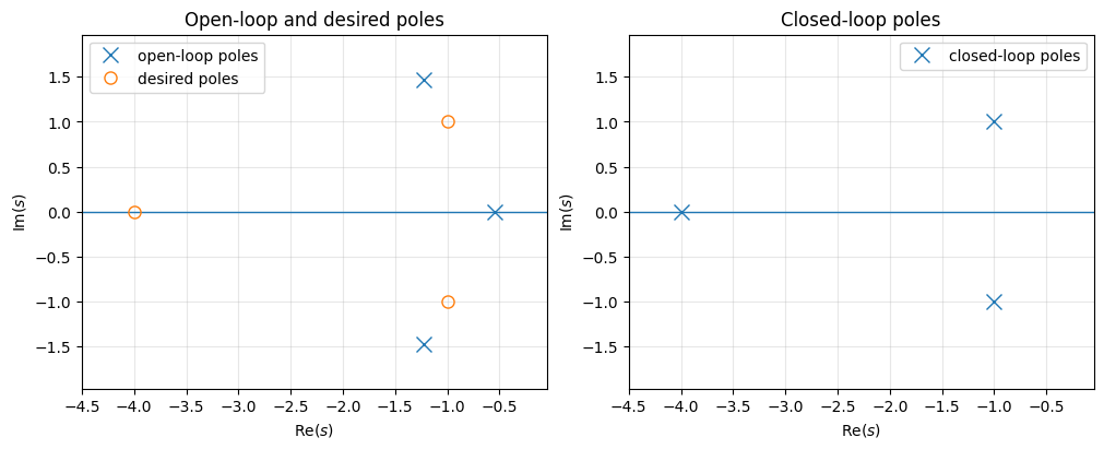
Suppose the desired closed-loop poles are \(-1\pm j\) and \(-4\). Then

\[ p_{\mathrm{des}}(s)=(s+1-j)(s+1+j)(s+4) =(s^2+2s+2)(s+4)=s^3+6s^2+10s+8. \]

Matching coefficients gives

\[\begin{split} \begin{aligned} 3+k_3 &= 6,\\ 5+k_2 &= 10,\\ 2+k_1 &= 8, \end{aligned} \qquad\Longrightarrow\qquad \begin{aligned} k_3&=3,\\ k_2&=5,\\ k_1&=6. \end{aligned} \end{split}\]

Thus,

\[ K=\begin{bmatrix}6&5&3\end{bmatrix}, \]

and the closed-loop characteristic polynomial satisfies

\[ \det(sI-A_{\mathrm{cl}})=p_{\mathrm{des}}(s). \]

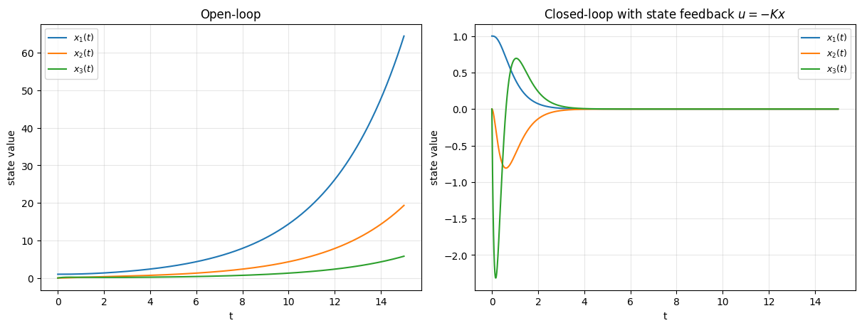
The following code snippet automates this process (which is also known as “pole placement.”)

K = [[6. 5. 3.]]
open-loop poles  = [-0.54660235+0.j         -1.22669883+1.46771151j -1.22669883-1.46771151j]
closed-loop poles = [-1.+1.j -1.-1.j -4.+0.j]

What if the system is not in controllable canonical form?

If the pair \((A,B)\) is controllable, then there exists an invertible matrix \(T\) such that under the coordinate change

\[ x = Tz \qquad\Longleftrightarrow\qquad z = T^{-1}x, \]

the dynamics become

\[ \dot z = A_c z + B_c u, \qquad A_c = T^{-1}AT,\quad B_c = T^{-1}B, \]

where \((A_c,B_c)\) is in controllable canonical form.

We will come back later to when such a \(T\) exists and how to compute it systematically. For now, we work through an example.

Take

\[\begin{split} A=\begin{bmatrix} 1&2&0\\ 0&1&1\\ 1&0&2 \end{bmatrix}, \qquad B=\begin{bmatrix} 0\\ 1\\ 1 \end{bmatrix}. \end{split}\]

One valid similarity transformation matrix is

\[\begin{split} T= \begin{bmatrix} -2&2&0\\ 1&-2&1\\ 3&-2&1 \end{bmatrix}, \qquad \det(T)=4\neq 0, \end{split}\]

and it satisfies

\[ T^{-1}AT = A_c,\qquad T^{-1}B=B_c. \]

Therefore, in the coordinates \(z=T^{-1}x\), the system has the controllable canonical form dynamics

\[ \dot z = A_c z + B_c u, \]

where

\[\begin{split} A_c=\begin{bmatrix} 0&1&0\\ 0&0&1\\ -a_0&-a_1&-a_2 \end{bmatrix} = \begin{bmatrix} 0&1&0\\ 0&0&1\\ 4&-5&4 \end{bmatrix}, \qquad B_c=\begin{bmatrix}0\\0\\1\end{bmatrix}. \end{split}\]

This observation leads to a practical state-feedback design procedure. Given a controllable pair \((A,B)\) and desired pole locations:

1. Find an invertible \(T\) such that \(A_c=T^{-1}AT\) and \(B_c=T^{-1}B\) are in controllable canonical form.

2. Design \(K_c\) in canonical coordinates so that \(\det(sI-(A_c-B_cK_c))=p_{\mathrm{des}}(s)\).

3. Transform back using \(K = K_cT^{-1}\), so that \(u=-Kx\) achieves the same closed-loop pole locations in the original coordinates.

Can we always tranform to the controllable canonical form?

Up to this pointwe have stated that this ability depends on whether the pair \((A,B)\) is controllable, but we have not given a formal definition of what this eans or how to check it.

Rather than introducing the definition, we will build intuition by examining a few simple examples. These examples illustrate, at a tructural level, why state feedback succeeds in some cases and fails in others.

An example where state feedback works (i.e., the system is controllable)

Consider the system

\[\begin{split} \dot x = \begin{bmatrix} 0 & 1\\ -2 & 1 \end{bmatrix} x + \begin{bmatrix} 0\\ 1 \end{bmatrix} u. \end{split}\]

Here, the control input appears directly in the second state equation, and the first state is coupled to the second through the system dynamics.

As a result, changes in the control input affect both states, either directly or indirectly. In such a situation, state feedback can influence all modes of the system, and it is possible to choose feedback gains to stabilize the closed-loop dynamics.

Indeed, by selecting an appropriate gain matrix \(K\), the eigenvalues of \(A-BK\) can be placed at desired locations.

An example where state feedback does not work (i.e., the system is not controllable)*

Consider the system

\[\begin{split} \dot x = \begin{bmatrix} -2 & 0\\ 0 & 1 \end{bmatrix} x + \begin{bmatrix} 2\\ 0 \end{bmatrix} u. \end{split}\]

The open-loop system has one stable mode (at \(-2\)) and one unstable mode (at \(+1\)).

Applying state feedback \(u=-Kx\) gives

\[\begin{split} \dot x = \begin{bmatrix} -2-2k_1 & 2k_2\\ 0 & 1 \end{bmatrix} x. \end{split}\]

Notice that the second state equation does not involve the control input. Consequently, the unstable mode at \(+1\) is completely unaffected by feedback.

No matter how the gains are chosen, this eigenvalue cannot be moved. Therefore, the system cannot be stabilized using state feedback.

Open-loop poles : [-4.   0.3 -1. ]
Desired poles   : [-2.+0.j -3.+0.j -6.+0.j]
Closed-loop poles: [-2. -3. -6.]
K = [[37.2 33.5  6.3]]

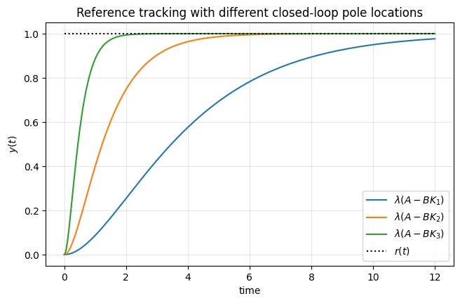
State feedback with feedforward

So far, we have focused on choosing a state-feedback gain \(K\) so that the closed-loop matrix \(A-BK\) has desired eigenvalues (and therefore desired stability and transient behavior).

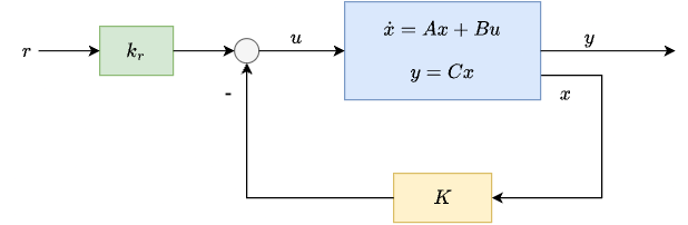
Now suppose we also have a reference input \(r\) that we want the output \(y\) to track.

Consider the state-space model

\[ \dot x(t)=Ax(t)+Bu(t), \qquad y(t)=Cx(t). \]

Use state feedback with a feedforward term

\[ u(t)=-Kx(t)+k_r\,r(t), \]

where \(K\in\mathbb{R}^{1\times n}\) is already chosen so that \(K\) stabilizes the closed-loop system, and \(k_r\in\mathbb{R}\) is a scalar we will choose to set the steady-state tracking behavior.

Substituting \(u(t)=-Kx(t)+k_r r(t)\) into \(\dot x=Ax+Bu\) gives

\[ \dot x(t) =Ax(t)+B\bigl(-Kx(t)+k_r r(t)\bigr) =(A-BK)x(t)+Bk_r\,r(t), \]

with output

\[ y(t)=Cx(t). \]

What can we do with the \(k_r\) term?

Consider a constant (step) reference \(r(t)=\bar r\) for \(t\ge 0\).

At steady state,

\[ y_{\mathrm{ss}} =Cx_{\mathrm{ss}} =-C(A-BK)^{-1}B\,k_r\,\bar r. \]

The steady-state gain from the reference \(\bar r\) to the output \(y_{\mathrm{ss}}\) is

\[ \frac{y_{\mathrm{ss}}}{\bar r} =-C(A-BK)^{-1}B\,k_r. \]

To enforce unit steady-state tracking (\(y_{\mathrm{ss}}=\bar r\)), choose

\[ k_r = -\frac{1}{C(A-BK)^{-1}B}, \]

provided \(C(A-BK)^{-1}B\neq 0\).

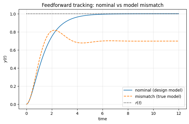
Feedforward control and model mismatch

In the previous example, we saw that adding a feedforward term \(k_r r(t)\) to the state-feedback controller allows us to enforce perfect steady-state tracking of a constant reference, provided the system model is known exactly.

This design relies on the quantity \(C(A-BK)^{-1}B\), which is computed using the assumed plant matrices \(A\) and \(B\). When these matrices accurately represent the true system, the feedforward gain \(k_r\) cancels the steady-state error and ensures \(y_{\mathrm{ss}}=r\).

However, this approach is inherently model-dependent. To illustrate this, consider the following setting:

• A nominal plant model \((A_{\mathrm{nom}},B_{\mathrm{nom}})\) is used to design the feedback gain \(K\) and the feedforward gain \(k_r\).

• The true plant \((A_{\mathrm{true}},B_{\mathrm{true}})\) differs slightly from the nominal model, representing modeling errors or parameter uncertainty.

• The same controller \(u=-Kx+k_r r\) is applied to both systems.

In the numerical example that follows, the feedforward controller achieves perfect steady-state tracking for the nominal model, but exhibits a steady-state tracking error when applied to the mismatched plant.

This highlights an important limitation of feedforward design: while it works well under nominal conditions, it is not robust to model uncertainties. This observation motivates the use of additional feedback mechanisms, such as integral action, to achieve robust reference tracking.

Designed on nominal model
K = [[6. 8.]]
k_r = 0.9999999999999991

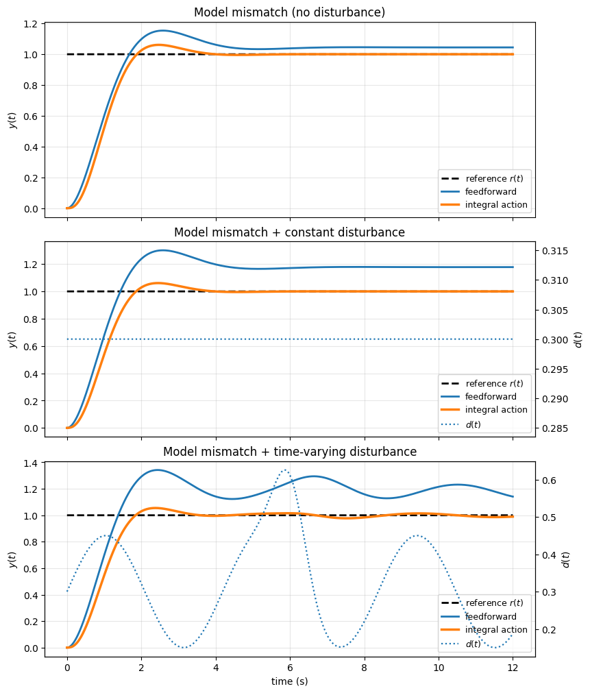
State feedback with integral action

We now introduce integral action as a way to address the robustness limitations of feedforward control.

Consider the linear system

\[ \dot x(t) = Ax(t) + Bu(t) + Ed(t), \qquad y(t) = Cx(t), \]

where \(x\in\mathbb{R}^n\), \(u\in\mathbb{R}\), \(d\in\mathbb{R}\), and \(y\in\mathbb{R}\).

We augment the state feedback controller with an integral term

\[ u(t) = -Kx(t) + k_i z(t), \]

where the additional state \(z\) integrates the tracking error:

\[ \dot z(t) = r(t) - y(t) = r(t) - Cx(t). \]

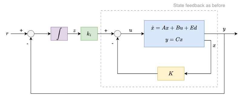
The key idea is that if a constant tracking error persists, then \(z(t)\) grows, which drives \(u(t)\) in a direction that reduces the error. This can eliminate steady-state errors caused by constant disturbances, model mismatch, or an incorrect feedforward gain.

Augmented system and state-feedback design with integral action

Define the augmented state

\[\begin{split} \bar x(t)=\begin{bmatrix}x(t)\\ z(t)\end{bmatrix}\in\mathbb{R}^{n+1}. \end{split}\]

Then the augmented dynamics can be written as

\[ \dot{\bar x}(t)=A_{\mathrm{aug}}\bar x(t)+B_{\mathrm{aug}}u(t) +E_{\mathrm{aug}}d(t)+R_{\mathrm{aug}}\,r(t), \]

with

\[\begin{split} A_{\mathrm{aug}}=\begin{bmatrix}A&0\\ -C&0\end{bmatrix},\qquad B_{\mathrm{aug}}=\begin{bmatrix}B\\ 0\end{bmatrix},\qquad E_{\mathrm{aug}}=\begin{bmatrix}E\\ 0\end{bmatrix},\qquad R_{\mathrm{aug}}=\begin{bmatrix}0\\ 1\end{bmatrix}. \end{split}\]

Substituting the control law \(u(t)=-Kx(t)+k_i z(t)\) gives

\[\begin{split} \dot{\bar x}(t) = \begin{bmatrix} A-BK & Bk_i\\ -C & 0 \end{bmatrix} \bar x(t) + E_{\mathrm{aug}}\,d(t) + R_{\mathrm{aug}}\,r(t). \end{split}\]

Now define the augmented feedback gain

\[ K_{\mathrm{aug}}=\begin{bmatrix}K & -k_i\end{bmatrix}. \]

Then the closed-loop augmented system can be written compactly as

\[ \dot{\bar x}(t) = \bigl(A_{\mathrm{aug}}-B_{\mathrm{aug}}K_{\mathrm{aug}}\bigr)\bar x(t) + E_{\mathrm{aug}}\,d(t) + R_{\mathrm{aug}}\,r(t). \]

Therefore, designing state feedback with integral action reduces to designing a state-feedback gain \(K_{\mathrm{aug}}\) for the augmented pair \((A_{\mathrm{aug}},B_{\mathrm{aug}})\).