All rights reserved. For enrolled students only. Redistribution prohibited.

Frequency response and transfer functions

What will we cover?

• Steady-state response under exponential and sinusoidal inputs

• Transfer functions

• Bode plots

• Poles and zeros (and eigenvalues)

• Block diagram algebra

Response of a linear system under sinusoidal inputs

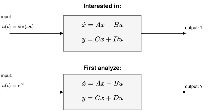
We are now interested in the response (solution) of a linear system

\[\begin{split}\begin{aligned} \dot{x} &= Ax + Bu \\ y &= Cx + Du \end{aligned}\end{split}\]

with \(A \in \mathbb{R}^{n \times n}, B \in \mathbb{R}^{n \times 1}, C \in \mathbb{R}^{1 \times n}\) and \(D \in \mathbb{R}\) under sinusoidal inputs, e.g., \(\sin(\omega t)\) or \(\cos(\omega t)\).

Instead we will first analyze the response under inputs of the form of

\[u(t) = \bar{u} e^{st}\]

with \(s \in \mathbb{C}\) and \(\bar{u} \in \mathbb{C}\).

Why care about \(e^{st}\)?

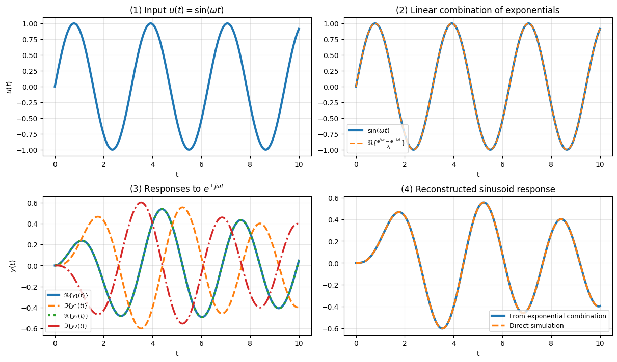
Exponentials generate sinusoids: Using Euler’s identity, \( e^{j\omega t} = \cos(\omega t) + j\sin(\omega t),\)we see that sinusoidal signals can be represented using complex exponentials.

Here is a concrete example.

\[ \sin(\omega t) = \frac{1}{2j}\left(e^{j\omega t} - e^{-j\omega t}\right). \]

Thus, a sinusoidal input is a linear combination of complex exponentials with

\[ s_1 = j\omega \quad \text{and} \quad s_2 = -j\omega. \]

Because the system is linear, if we know the response to \(e^{s_1 t}\) and \(e^{s_2 t}\), then we automatically know the response to any linear combination:

\[ \alpha e^{s_1 t} + \beta e^{s_2 t}. \]

Thus, by understanding exponential inputs, we can understand a wide range of signals, including:

• sinusoids,

• damped oscillations,

• and combinations of oscillatory modes.

Response to an exponential input

Assume that all eigenvalues \(\lambda_i\) of \(A\) satisfy

\[ \text{Re}(\lambda_i) < 0. \]

Consider an exponential input of the form

\[ u(t) = \bar u\, e^{s t}, \]

where \(\bar u \in \mathbb{C}\) and \(s \neq \lambda_i(A)\) for all \(i\).

The state solution is

\[ x(t) = e^{At} x_0 + \int_0^t e^{A(t-\tau)} B u(\tau)\, d\tau. \]

Substituting \(u(\tau) = \bar u e^{s\tau}\) gives

\[ x(t) = e^{At} x_0 + \int_0^t e^{A(t-\tau)} B \bar u e^{s\tau}\, d\tau. \]

Factor out \(e^{At}\):

\[ x(t) = e^{At} x_0 + e^{At} \left( \int_0^t e^{-A\tau} e^{s\tau} d\tau \right) B \bar u.\]

Combine exponentials

\[ e^{-A\tau} e^{s\tau} = e^{(sI - A)\tau}. \]

Thus,

\[ x(t) = e^{At} x_0 + e^{At} \left( \int_0^t e^{(sI-A)\tau} d\tau \right) B \bar u. \]

Since \(sI - A\) is invertible (because \(s\) is not an eigenvalue of \(A\)),

\[ \int_0^t e^{(sI-A)\tau} d\tau = (sI-A)^{-1}\!\left(e^{(sI-A)t} - I\right). \]

Substituting back,

\[ x(t) = e^{At} x_0 + e^{At} (sI-A)^{-1} \left(e^{(sI-A)t} - I\right) B \bar u. \]

Using \(e^{At} e^{(sI-A)t} = e^{s t},\) we obtain

\[ x(t) = e^{At}\!\left(x_0 - (sI-A)^{-1}B\bar u\right) + (sI-A)^{-1}B\bar u\, e^{s t}. \]

With \(y(t) = Cx(t) + D u(t)\), we get

\[ y(t) = C e^{At}\!\left(x_0 - (sI-A)^{-1}B\bar u\right) + C(sI-A)^{-1}B\bar u\, e^{s t} + D\bar u\, e^{s t}. \]

Steady-state response under exponential inputs

Because the system is stable, the term involving \(e^{At}\) decays to zero as time increases.

At steady state, only the forced term remains. Therefore,

\[ y_{\text{ss}}(t) = \left(C(sI-A)^{-1}B + D\right)\bar{u}\, e^{s t}. \]

For stable linear systems,

\[ u(t) = \bar{u} e^{s t} \quad \Longrightarrow \quad y_{\text{ss}}(t) = G(s)\,\bar{u}\, e^{s t}, \]

where

\[ G(s) = C(sI-A)^{-1}B + D. \]

This function (of s) is call the transfer function for the system.

Observations:

• The steady-state output has the same exponential form as the input.

• The system acts as a complex gain evaluated at \(s\).

Example: Damped linear oscillator

Consider the second-order system written in state-space form

\[ \dot x(t)=Ax(t)+Bu(t), \qquad y(t)=Cx(t), \]

with

\[\begin{split} A=\begin{bmatrix} 0 & \omega_0\\ -\omega_0 & -2\zeta\omega_0 \end{bmatrix}, \qquad B=\begin{bmatrix} 0\\ k\,\omega_0 \end{bmatrix}, \qquad C=\begin{bmatrix} 1 & 0 \end{bmatrix}, \qquad D=0. \end{split}\]

For \(\zeta>0\), this is a stable damped oscillator.

The transfer function from \(u\) to \(y\) is

\[\begin{split} \begin{aligned} G_{uy}(s) &= C(sI-A)^{-1}B + D \\[6pt] &= [\,1\;0\,] \left( \frac{1}{s^2+2\zeta\omega_0 s+\omega_0^2} \begin{bmatrix} s+2\zeta\omega_0 & \omega_0 \\ -\omega_0 & s \end{bmatrix} \right) \begin{bmatrix} 0\\ k\omega_0 \end{bmatrix} \\[10pt] &= \frac{k\omega_0^2}{s^2+2\zeta\omega_0 s+\omega_0^2}. \end{aligned} \end{split}\]

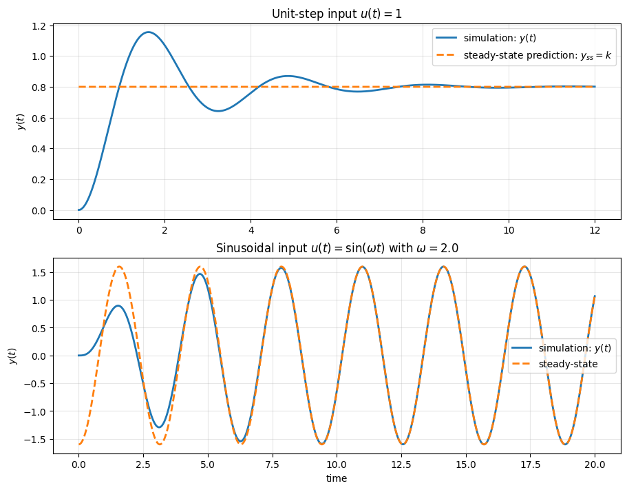
A unit step is the exponential input with \(s=0\) (since \(e^{0t}=1\)), so the steady-state output is

\[ y_{\text{ss}} = G_{uy}(0)\cdot 1 = k. \]

Write

\[ u(t)=\sin(\omega t) =\frac{1}{2}\Bigl(j e^{-j\omega t}-j e^{j\omega t}\Bigr). \]

By linearity, the steady-state output is the same linear combination of the corresponding steady-state responses:

\[ y_{\text{ss}}(t) = \frac{1}{2}\Bigl( jG_{uy}(-j\omega)e^{-j\omega t} - jG_{uy}(j\omega)e^{j\omega t} \Bigr). \]

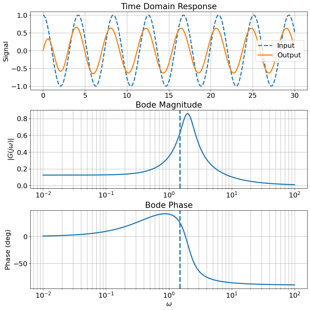
Below, we compute both the simulated response and the predicted steady-state response, and plot them together.

Steady-state response to sinusoidal inputs

Consider a stable linear time-invariant system with transfer function \(G(s)\). Let the input be

\[ u(t) = A_u \cos(\omega t). \]

Using Euler’s identity,

\[ \cos(\omega t) = \text{Re}\{e^{j\omega t}\}, \]

we can write

\[ u(t) = \text{Re}\{A_u e^{j\omega t}\}. \]

Because the system is linear and stable, the steady-state response to the complex exponential input

\[ A_u e^{j\omega t} \]

is

\[ G(j\omega) A_u e^{j\omega t}. \]

Taking the real part gives the steady-state output:

\[ y_{\mathrm{ss}}(t) = \text{Re}\{ G(j\omega) A_u e^{j\omega t} \}. \]

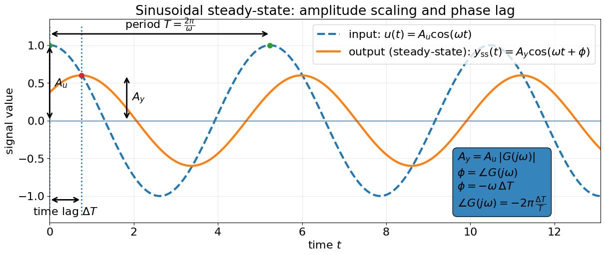
Now write

\[ G(j\omega) = |G(j\omega)| e^{j \angle G(j\omega)}. \]

Then

\[ y_{\mathrm{ss}}(t) = \text{Re}\{ A_u |G(j\omega)| e^{j(\omega t + \angle G(j\omega))} \} = A_u |G(j\omega)| \cos\!\left(\omega t + \angle G(j\omega)\right). \]

Thus, the output sinusoid has:

• the same frequency \(\omega\),

• amplitude scaled by \(|G(j\omega)|\),

• and phase shift \(\angle G(j\omega)\).

\[\begin{split} \begin{aligned} \sin(\omega t) &\;\rightarrow\; |G(j\omega)|\,\sin(\omega t + \angle G(j\omega)) \\ \cos(\omega t) &\;\rightarrow\; |G(j\omega)|\,\cos(\omega t + \angle G(j\omega)) \\ 1 &\;\rightarrow\; G(0) = D - C A^{-1} B \end{aligned} \end{split}\]

Aircraft Pitch Model

We now consider the longitudinal pitch dynamics model presented in the University of Michigan Control Tutorials for MATLAB and Simulink (CTMS):

https://ctms.engin.umich.edu/CTMS/?example=AircraftPitch&section=SystemModeling

The model represents small perturbations about steady cruise flight and describes the pitch motion of an aircraft.

Under standard linearization assumptions (small angles, constant speed, decoupled longitudinal dynamics), the system is written in terms of:

• \(\alpha\) : angle of attack

• \(q\) : pitch rate

• \(\theta\) : pitch angle

The control input is the elevator deflection \(\delta\).

The longitudinal pitch model is

\[ \dot{\alpha} = \mu\Omega\sigma\!\left[ -(C_L + C_D)\alpha + \frac{1}{\mu - C_L} q - (C_W \sin\gamma)\theta + C_L \right], \]

\[ \dot{q} = \frac{\mu\Omega}{2J_{yy}} \left[ C_M - \eta(C_L + C_D)\alpha + C_M + \sigma C_M(1-\mu C_L) q + (\eta C_W \sin\gamma)\delta \right], \]

\[ \dot{\theta} = \Omega q. \]

For this model:

• The input is the elevator deflection \(\delta\).

• The output is the pitch angle \(\theta\).

We may express the linearized system compactly as

\[ \dot{x}(t) = A x(t) + B \delta(t), \qquad y(t) = C x(t), \]

with

\[\begin{split} x(t) = \begin{bmatrix} \alpha(t) \\ q(t) \\ \theta(t) \end{bmatrix} \end{split}\]

and

\[\begin{split} A = \begin{bmatrix} -0.313 & 56.7 & 0 \\ -0.0139 & -0.426 & 0 \\ 0 & 56.7 & 0 \end{bmatrix}, \qquad B = \begin{bmatrix} 0.232 \\ 0.0203 \\ 0 \end{bmatrix}, \end{split}\]

\[ C = \begin{bmatrix} 0 & 0 & 1 \end{bmatrix}, \qquad D = \begin{bmatrix} 0 \end{bmatrix}. \]

Hence

\[ G_{\delta\to\theta}(s) = C(sI-A)^{-1}B. \]

Compute

\[\begin{split} sI-A = \begin{bmatrix} s+0.313 & -56.7 & 0 \\ 0.0139 & s+0.426 & 0 \\ 0 & -56.7 & s \end{bmatrix}. \end{split}\]

Therefore,

\[\begin{split} G_{\delta\to\theta}(s) = \begin{bmatrix}0&0&1\end{bmatrix} (sI-A)^{-1} \begin{bmatrix} 0.232 \\ 0.0203 \\ 0 \end{bmatrix}. \end{split}\]

Carrying out the matrix multiplication (and using \(D=0\)) yields a third-order transfer function

\[ G_{\delta\theta}(s) = \frac{1.151s + 0.177}{s\left(s^2+0.739s+0.921\right)}. \]

Shortcuts for obtaining the transfer function

Consider a linear time-invariant input–output system written in ODE form:

\[ \frac{d^n y}{dt^n} + a_1 \frac{d^{n-1} y}{dt^{n-1}} + \cdots + a_n y = b_0 \frac{d^m u}{dt^m} + b_1 \frac{d^{m-1} u}{dt^{m-1}} + \cdots + b_m u, \]

where \(y(t)\) is the output and \(u(t)\) is the input.

Key observations

• For linear systems, if the input is an exponential

\[ u(t) = e^{st}, \]

then at steady state the output must also be of the form

\[ y_{ss}(t) = y_0 e^{st}, \]

for some scalar \(y_0\) (provided \(s\) is not a root of the characteristic polynomial \(s^n + a_1 s^{n-1} + \cdots + a_n\)).

• If \(u(t) = e^{st}\), then

\[ \frac{d^k u}{dt^k} = s^k e^{st}, \]

and similarly,

\[ \frac{d^k y_{ss}}{dt^k} = y_0 s^k e^{st}. \]

Plugging \(u(t)=e^{st}\) and \(y_{ss}(t)=y_0 e^{st}\) into the differential equation gives

\[ \left( s^n + a_1 s^{n-1} + \cdots + a_n \right) y_0 e^{st} = \left( b_0 s^m + b_1 s^{m-1} + \cdots + b_m \right) e^{st}. \]

Cancel \(e^{st}\):

\[ \left( s^n + a_1 s^{n-1} + \cdots + a_n \right) y_0 = b_0 s^m + b_1 s^{m-1} + \cdots + b_m. \]

Solving for \(y_0\),

\[ y_0 = \frac{b_0 s^m + b_1 s^{m-1} + \cdots + b_m} {s^n + a_1 s^{n-1} + \cdots + a_n}. \]

Since \(y_{ss}(t) = y_0 e^{st}\) and \(u(t)=e^{st}\), we obtain

\[ \boxed{ G(s) = \frac{b(s)}{a(s)} = \frac{b_0 s^m + b_1 s^{m-1} + \cdots + b_m} {s^n + a_1 s^{n-1} + \cdots + a_n}. } \]

The denominator \(a(s)\) is the characteristic polynomial of the ODE (or, in short, of the system).

Examples: ODE ↔ Transfer Function

In the following examples, substitute \(y_{ss} = y_0 e^{st}\), \(u = e^{st}\) in the given ODEs and isolate \(y_0\) to obtain an expression for the transfer function from \(y\) to \(y\).

1. Integrator: \( \dot y = u.\)

\[ s y_0 e^{st} = e^{st} \Rightarrow G(s) = \frac{1}{s}. \]

2. Derivative: \( y = \dot u.\)

\[ y_0 e^{st} = s e^{st} \Rightarrow G(s) = s. \]

3. First-order system: \( \dot y + a y = u.\)

\[ s y_0 e^{st} + a y_0 e^{st} = e^{st} \Rightarrow G(s) = \frac{1}{s + a}. \]

4. Double integrator: \( \ddot y = u.\)

\[ s^2 y_0 e^{st} = e^{st} \Rightarrow G(s) = \frac{1}{s^2}. \]

5. Second-order system: \( \ddot y + 2\zeta\omega_n \dot y + \omega_n^2 y = u.\)

\[ \left( s^2 + 2\zeta\omega_n s + \omega_n^2 \right) y_0 e^{st} = e^{st} \Rightarrow G(s) = \frac{1}{s^2 + 2\zeta\omega_n s + \omega_n^2}. \]

6. PID controller: \( y = k_p u + k_d \dot u + k_i \int u\,dt.\)

\[ y_0 e^{st} = k_p e^{st} + k_d s e^{st} + k_i \frac{1}{s} e^{st} \]

\[ G(s) = k_p + k_d s + \frac{k_i}{s} = \frac{k_d s^2 + k_p s + k_i}{s}. \]

Example: Linearized balance system

Consider the linearized model of a cart–pendulum (balance) system with the variables

• \(p\) = cart position

• \(\theta\) = pendulum angle

• \(F\) = applied force .

The linearized differential equations are

\[ M\ddot p - m\ell \ddot\theta + c \dot p = F, \]

\[ J\ddot\theta - m\ell \ddot p + \gamma \dot\theta - m g \ell \theta = 0. \]

Here \(M, m, \ell, J, c, \gamma, g\) are physical parameters.

If the input is of the form

\[ F(t) = e^{st}, \]

then all signals will reach steady-state of the form

\[ p(t)=P e^{st}, \qquad \theta(t)=\Theta e^{st}. \]

Substituting into the ODEs gives

\[ M s^2 P - m\ell s^2 \Theta + c s P = 1, \]

\[ J s^2 \Theta - m\ell s^2 P + \gamma s \Theta - m g \ell \Theta = 0. \]

Rearrange:

\[ (M s^2 + c s)P - m\ell s^2 \Theta = 1, \]

\[ - m\ell s^2 P + (J s^2 + \gamma s - m g \ell)\Theta = 0. \]

This can be written compactly as

\[\begin{split} \begin{bmatrix} M s^2 + c s & -m\ell s^2 \\ - m\ell s^2 & J s^2 + \gamma s - m g \ell \end{bmatrix} \begin{bmatrix} P \\ \Theta \end{bmatrix} = \begin{bmatrix} 1 \\ 0 \end{bmatrix}. \end{split}\]

Let

\[ \Delta(s) = (M s^2 + c s)(J s^2 + \gamma s - m g \ell) - (m\ell s^2)^2. \]

Expanding gives

\[ \Delta(s) = (MJ - m^2\ell^2)s^4 + (\gamma M + cJ)s^3 + (c\gamma - M m g \ell)s^2 - c m g \ell s. \]

The transfer function from force \(F\) to angle \(\theta\)

\[ \Theta(s) = \frac{m\ell s^2}{\Delta(s)}. \]

\[ H_{F\to\theta}(s) = \frac{m\ell s^2} {(MJ - m^2\ell^2)s^4 + (\gamma M + cJ)s^3 + (c\gamma - M m g \ell)s^2 - c m g \ell s}. \]

The transfer function from force \(F\) to position \(p\)

\[ P(s) = \frac{J s^2 + \gamma s - m g \ell} {\Delta(s)}. \]

\[ H_{F\to p}(s) = \frac{J s^2 + \gamma s - m g \ell} {(MJ - m^2\ell^2)s^4 + (\gamma M + cJ)s^3 + (c\gamma - M m g \ell)s^2 - c m g \ell s}. \]

Transfer function from F to theta:
                              l⋅m⋅s                              
─────────────────────────────────────────────────────────────────
     3        2                    2                      2  2  3
J⋅M⋅s  + J⋅c⋅s  - M⋅g⋅l⋅m⋅s + M⋅γ⋅s  - c⋅g⋅l⋅m + c⋅γ⋅s - l ⋅m ⋅s 

Transfer function from F to p:
                            2                                        
                         J⋅s  - g⋅l⋅m + γ⋅s                          
─────────────────────────────────────────────────────────────────────
  ⎛     3        2                    2                      2  2  3⎞
s⋅⎝J⋅M⋅s  + J⋅c⋅s  - M⋅g⋅l⋅m⋅s + M⋅γ⋅s  - c⋅g⋅l⋅m + c⋅γ⋅s - l ⋅m ⋅s ⎠

Common denominator Δ(s):
     3        2                    2                      2  2  3
J⋅M⋅s  + J⋅c⋅s  - M⋅g⋅l⋅m⋅s + M⋅γ⋅s  - c⋅g⋅l⋅m + c⋅γ⋅s - l ⋅m ⋅s 

Expanded denominator:
     3        2                    2                      2  2  3
J⋅M⋅s  + J⋅c⋅s  - M⋅g⋅l⋅m⋅s + M⋅γ⋅s  - c⋅g⋅l⋅m + c⋅γ⋅s - l ⋅m ⋅s 

--- Direct determinant method ---
G_theta:
<TransferFunction>: sys[30]
Inputs (1): ['u[0]']
Outputs (1): ['y[0]']

                     0.1 s^2
  ----------------------------------------------
  -0.004 s^4 + 0.0506 s^3 - 0.976 s^2 - 0.0981 s

G_p:
<TransferFunction>: sys[31]
Inputs (1): ['u[0]']
Outputs (1): ['y[0]']

            0.006 s^2 + 0.05 s - 0.981
  ----------------------------------------------
  -0.004 s^4 + 0.0506 s^3 - 0.976 s^2 - 0.0981 s

--- State-space method ---
G_theta:
<TransferFunction>: sys[35]
Inputs (1): ['u[0]']
Outputs (1): ['y[0]']

       -2.487e-14 s^2 - 25 s
  -------------------------------
  s^3 - 12.65 s^2 + 244 s + 24.52

G_p:
<TransferFunction>: sys[37]
Inputs (1): ['u[0]']
Outputs (1): ['y[0]']

  -1.599e-14 s^3 - 1.5 s^2 - 12.5 s + 245.2
  -----------------------------------------
     s^4 - 12.65 s^3 + 244 s^2 + 24.52 s

Poles and zeros of a transfer function

If a transfer function is written as

\[ G(s) = \frac{b(s)}{a(s)}, \]

then

• Zeros of \(G\) are the roots of

  \[ b(s) = 0, \]

• Poles of \(G\) are the roots of

  \[ a(s) = 0. \]

Example

Consider the transfer function

\[ G(s) = \frac{s + 2}{s^2 + 4s + 5}. \]

The zeros are the roots of the numerator

\[ s + 2 = 0 \quad \Longrightarrow \quad s = -2. \]

The poles are the roots of the denominator

\[ s^2 + 4s + 5 = 0, \]

i.e.,

\[ s = \frac{-4 \pm \sqrt{16 - 20}}{2} = -2 \pm j. \]

Example

Consider the transfer function

\[ G(s) = \frac{s + 2}{s^2 + 3s + 2}. \]

The zeros are the roots of the numerator

\[ s + 2 = 0 \quad \Longrightarrow \quad s = -2. \]

The poles are the roots of the denominator

\[ s^2 + 3s + 2 = 0. \]

Factor:

\[ (s+1)(s+2) = 0, \]

so

\[ s = -1, \quad s = -2. \]

Notice that the factor \((s+2)\) appears in both the numerator and denominator. This means there is a “pole–zero cancellation” at \(s = -2\).

After cancellation, the transfer function becomes

\[ G(s) = \frac{1}{s+1}. \]

Poles and Eigenvalues

Consider a state-space model

\[ \dot{x}(t) = A x(t) + B u(t), \qquad y(t) = C x(t) + D u(t), \]

with transfer function

\[ G(s) = C (sI - A)^{-1} B + D. \]

Using the identity

\[ (sI - A)^{-1} = \frac{1}{\det(sI - A)} \, \operatorname{adj}(sI - A), \]

we can write

\[ G(s) = C \left( \frac{1}{\det(sI - A)} \operatorname{adj}(sI - A) \right) B + D. \]

Therefore, the denominator of \(G(s)\) is given by

\[ a(s) = \det(sI - A). \]

By definition, the eigenvalues of \(A\) are the roots of

\[ \det(sI - A) = 0. \]

Hence,

\[ \boxed{ \text{poles of } G(s) \text{ are the eigenvalues of } A } \]

In general, this statement holds up to possible cancellations between the numerator and denominator. When no such cancellations occur, the poles of the transfer function exactly match the eigenvalues of \(A\).

Interpretation

• The matrix \(A\) determines the internal dynamics of the system.

• The eigenvalues of \(A\) determine how the state evolves.

• These same values appear as the poles of the transfer function, which determine the input–output behavior.

Thus, poles provide a direct link between state-space dynamics and transfer-function representations.

Example

Consider the state-space system

\[\begin{split} \dot{x}(t) = \begin{bmatrix} -1 & 0 \\ 0 & -2 \end{bmatrix} x(t) + \begin{bmatrix} 1 \\ 1 \end{bmatrix} u(t), \qquad y(t) = \begin{bmatrix} 1 & 1 \end{bmatrix} x(t), \qquad D = 0. \end{split}\]

The eigenvalues of \(A\) are

\[ \lambda_1 = -1, \qquad \lambda_2 = -2. \]

Compute

\[ G(s) = C (sI - A)^{-1} B: \]

We have

\[\begin{split} (sI - A) = \begin{bmatrix} s+1 & 0 \\ 0 & s+2 \end{bmatrix}, \qquad (sI - A)^{-1} = \begin{bmatrix} \frac{1}{s+1} & 0 \\ 0 & \frac{1}{s+2} \end{bmatrix}. \end{split}\]

Thus

\[\begin{split} (sI - A)^{-1} B = \begin{bmatrix} \frac{1}{s+1} \\ \frac{1}{s+2} \end{bmatrix}. \end{split}\]

Multiplying by \(C\),

\[ G(s) = \frac{1}{s+1} + \frac{1}{s+2}. \]

Combine into a single fraction:

\[ G(s) = \frac{(s+2) + (s+1)}{(s+1)(s+2)} = \frac{2s + 3}{(s+1)(s+2)}. \]

Recap:

• Eigenvalues of \(A\): \(-1\), \(-2\)

• Poles of \(G(s)\): \(-1\), \(-2\)

Example

Consider the state-space system

\[\begin{split} \dot{x}(t) = \begin{bmatrix} -1 & 0 \\ 0 & -2 \end{bmatrix} x(t) + \begin{bmatrix} 1 \\ 0 \end{bmatrix} u(t), \qquad y(t) = \begin{bmatrix} 1 & 0 \end{bmatrix} x(t). \end{split}\]

The matrix \(A\) has the eigenvalues \(-1\) and \(-2\).

Transfer function (after a pole-zero cancellation) is

\[ G(s) = \frac{1}{s+1}, \]

which has only one pole at \(s=-1\).

Steady-state gain for step inputs using the transfer function

Consider a linear input–output system written in ODE form:

\[ \frac{d^n y}{dt^n} + a_1 \frac{d^{n-1} y}{dt^{n-1}} + \cdots + a_n y = b_0 \frac{d^m u}{dt^m} + b_1 \frac{d^{m-1} u}{dt^{m-1}} + \cdots + b_m u. \]

The corresponding transfer function is

\[ G(s) = \frac{b(s)}{a(s)} = \frac{b_0 s^m + b_1 s^{m-1} + \cdots + b_m} {s^n + a_1 s^{n-1} + \cdots + a_n}. \]

Now suppose the input is a constant (step) input

\[ u(t) = \bar{u}. \]

If the system is stable, then the output converges to a constant steady-state value

\[ y(t) = \bar{y}. \]

At steady state, all derivatives of \(y(t)\) are zero, and all derivatives of \(u(t)\) of order \(1\) or higher are also zero. Substituting into the ODE gives

\[ a_n \bar{y} = b_m \bar{u}. \]

Therefore,

\[ \frac{\bar{y}}{\bar{u}} = \frac{b_m}{a_n}. \]

This ratio is the steady-state gain from a step input to the output.

Evaluating the transfer function at \(s=0\) gives

\[ G(0) = \frac{b_m}{a_n}. \]

Therefore, for a stable system, the steady-state gain from a constant input to the output is

\[ G(0). \]

If the same system is written in state-space form

\[ \dot{x}(t) = A x(t) + B u(t), \qquad y(t) = C x(t) + D u(t), \]

then

\[ G(s) = C(sI-A)^{-1}B + D. \]

Evaluating at \(s=0\) gives

\[ G(0) = D - C A^{-1} B. \]

Thus, for a stable system, the steady-state gain from a step input to the output is

\[ D - C A^{-1} B. \]

Block diagram algebra

Transfer functions combine in simple ways under standard block-diagram interconnections.

We will consider three different basic interconnections.

Serial interconnection

Suppose two systems are connected in series:

\[ u \;\longrightarrow\; G_1(s) \;\longrightarrow\; G_2(s) \;\longrightarrow\; y. \]

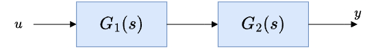
If the input is \(u(t)=e^{st}\), then the output of the first block is

\[ G_1(s)e^{st}, \]

and the output of the second block is

\[ G_2(s)\,G_1(s)e^{st}. \]

Therefore, the overall transfer function from \(u\) to \(y\) is

\[ G_{u\to y}(s)=G_2(s)\,G_1(s). \]

Parallel interconnection

Suppose the same input \(u\) is applied to two systems in parallel, and the outputs are added:

\[ u \;\longrightarrow\; G_1(s), \qquad u \;\longrightarrow\; G_2(s), \qquad y = y_1 + y_2. \]

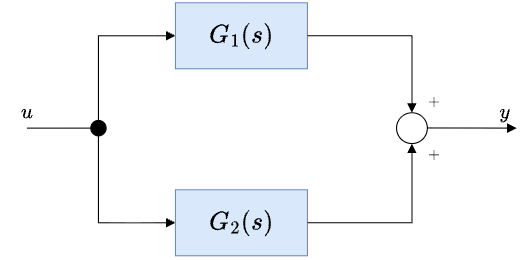
If \(u(t)=e^{st}\), then

\[ y_1(t)=G_1(s)e^{st}, \qquad y_2(t)=G_2(s)e^{st}. \]

Hence,

\[ y(t) = \bigl(G_1(s)+G_2(s)\bigr)e^{st}. \]

Therefore, the overall transfer function is

\[ G_{u\to y}(s)=G_1(s)+G_2(s). \]

Feedback interconnection

Consider the feedback interconnection

\[ e = u - G_2(s)y, \qquad y = G_1(s)e. \]

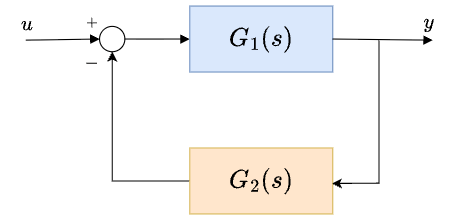
Substituting the error signal into the forward path gives

\[ y = G_1(s)\bigl(u - G_2(s)y\bigr). \]

Rearranging,

\[ y + G_1(s)G_2(s)y = G_1(s)u, \]

so

\[ \bigl(1+G_1(s)G_2(s)\bigr)y = G_1(s)u. \]

Therefore, the closed-loop transfer function from \(u\) to \(y\) is

\[ G_{u\to y}(s)=\frac{G_1(s)}{1+G_1(s)G_2(s)}. \]

Example (of block diagram algebra)

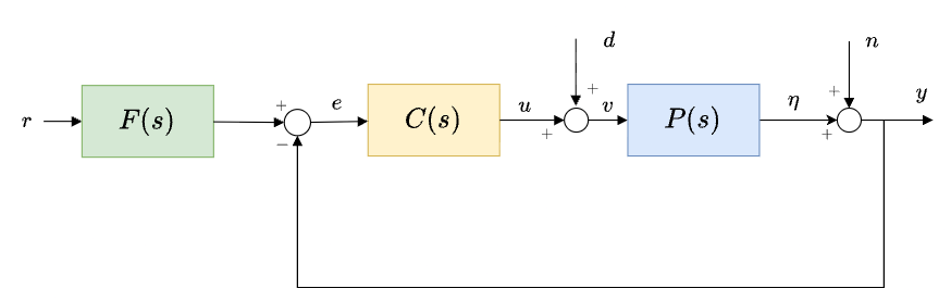
We proceed by following the signals in the block diagram step by step.

From the first summing junction,

\[ e = F r - y. \]

From the diagram:

• Controller:

\[ u = C e \]

• Disturbance enters before the plant:

\[ v = u + d \]

• Plant output (before measurement noise):

\[ \eta = P v \]

• Measurement noise:

\[ y = \eta + n \]

Start from

\[ y = \eta + n = P v + n. \]

Substitute \(v = u + d\):

\[ y = P(u + d) + n = P u + P d + n. \]

Now substitute \(u = C e\):

\[ y = P C e + P d + n. \]

Recall

\[ e = F r - y. \]

Substitute \(y\):

\[ e = F r - (P C e + P d + n). \]

Expand:

\[ e = F r - P C e - P d - n. \]

Group terms:

\[ e + P C e = F r - n - P d. \]

\[ (1 + P C)e = F r - n - P d. \]

Divide through:

\[ e = \frac{F}{1+PC} \, r - \frac{1}{1+PC} \, n - \frac{P}{1+PC} \, d. \]

The error is composed of three contributions:

\[ e = G_{r \to e} \, r + G_{n \to e} \, n + G_{d \to e} \, d \]

where

\[ G_{r \to e} = \frac{F}{1+PC}, \qquad G_{n \to e} = -\frac{1}{1+PC}, \qquad G_{d \to e} = -\frac{P}{1+PC}. \]

Important observation:

The term \(\frac{1}{1+PC}\) appears in all closed-loop transfer functions.

Example

For the system shown, compute the transfer functions

• from \(u\) to \(y\),

• from \(u\) to \(w\).

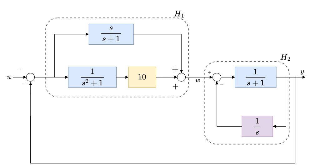
We will use the intermediate subsystems \(H_1\) and \(H_2\) to simplify the derivation.

Compute \(H_1\)

The subsystem \(H_1\) has two parallel branches from its input to the signal \(w\):

• upper branch:

\[ \frac{s}{s+1}, \]

• lower branch:

\[ \frac{10}{s^2+1}. \]

Since these two branches are in parallel,

\[ H_1(s)=\frac{s}{s+1}+\frac{10}{s^2+1}. \]

This can be written over a common denominator as

\[ H_1(s) = \frac{s(s^2+1)+10(s+1)}{(s+1)(s^2+1)} = \frac{s^3+11s+10}{(s+1)(s^2+1)}. \]

Compute \(H_2\)

The subsystem \(H_2\) is a negative-feedback interconnection with

• forward path:

\[ G(s)=\frac{1}{s+1}, \]

• feedback path:

\[ H(s)=\frac{1}{s}. \]

Therefore,

\[ H_2(s) = \frac{G(s)}{1+G(s)H(s)} = \frac{\frac{1}{s+1}}{1+\frac{1}{s+1}\frac{1}{s}}. \]

Simplifying,

\[ H_2(s) = \frac{\frac{1}{s+1}}{\frac{s(s+1)+1}{s(s+1)}} = \frac{s}{s^2+s+1}. \]

Outer feedback loop

Once \(H_1\) and \(H_2\) are computed, the overall diagram can be simplified to the following feedback interconnection.

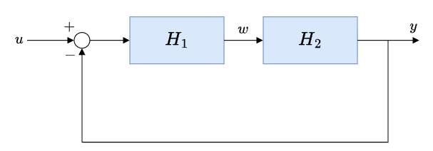
The transfer function from \(u\) to \(y\) is then

\[ \frac{H_1(s)H_2(s)}{1+H_1(s)H_2(s)} =\frac{s^5 + 11s^2 + 10s} {s^5 + 3s^4 + 3s^3 + 14s^2 + 12s + 1}. \]

Similarly, the transfer function from \(u\) to \(w\) is

\[ \frac{H_1(s)}{1+H_1(s)H_2(s)} = \frac{s^5 + s^4 + 12s^3 + 21s^2 + 21s + 10} {s^5 + 3s^4 + 3s^3 + 14s^2 + 12s + 1}. \]