Nyquist plot and criteria plus Margins

What are we going to cover?

• Graphical representations of transfer functions

• Bode and Nyquist plots

• Nyquist stability criterion

• Robustness margins

##Graphical representations of transfer functions

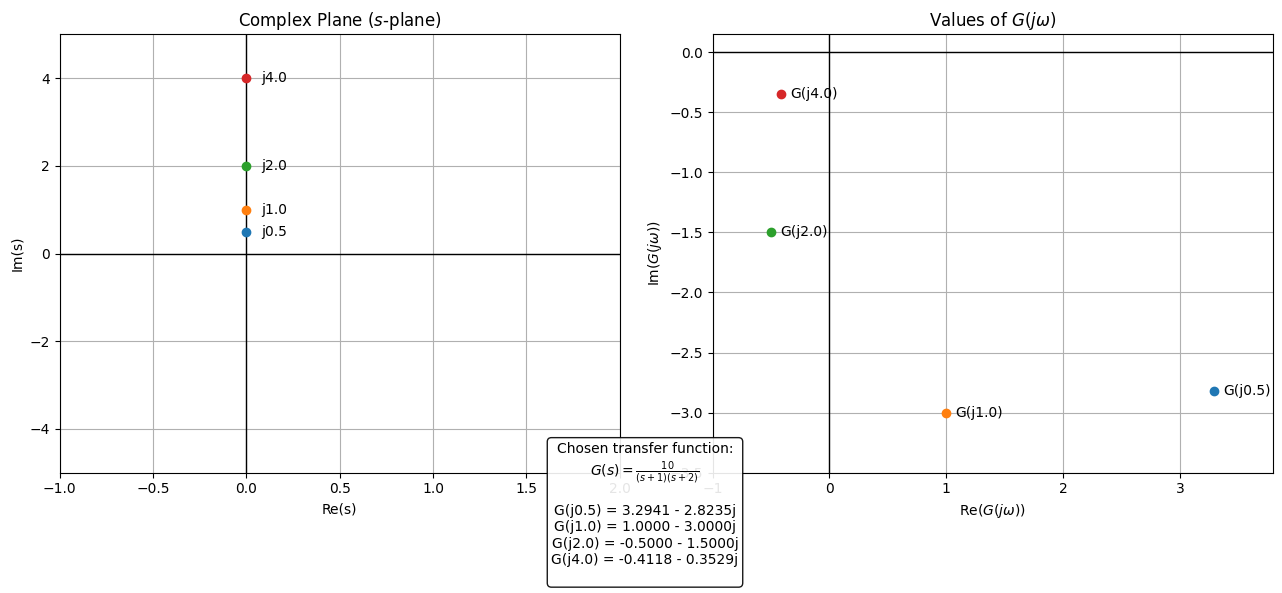
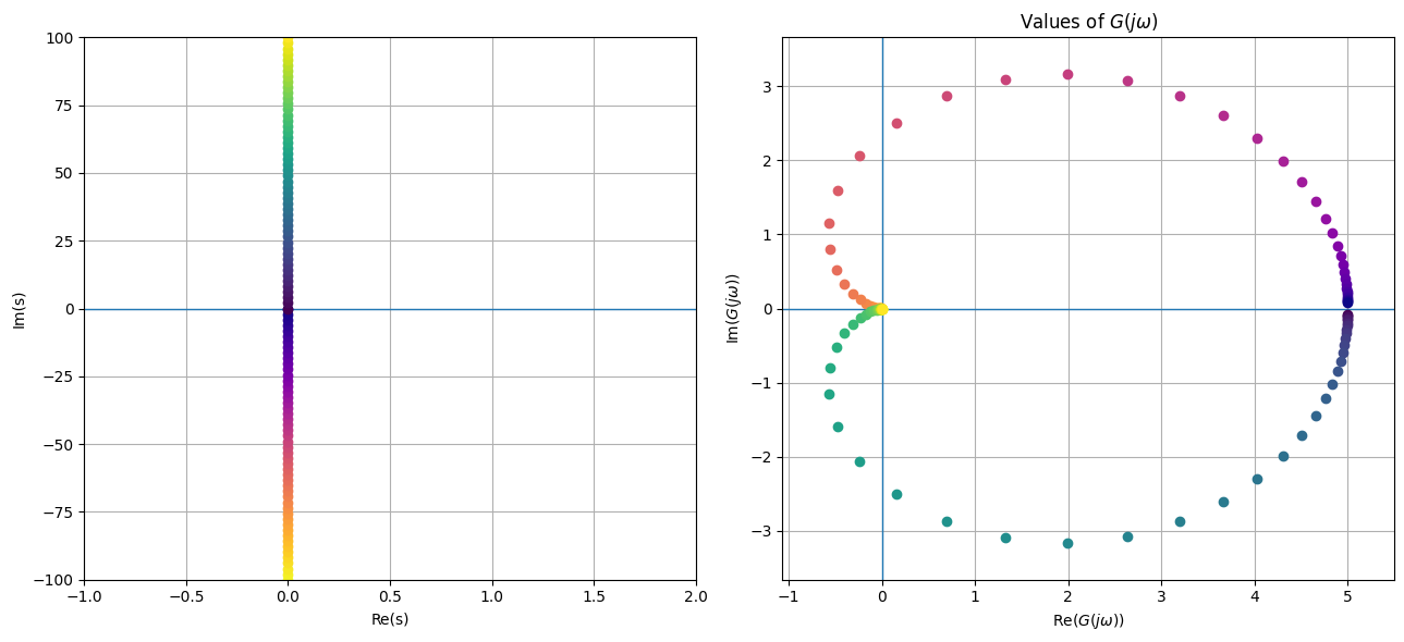
A transfer function \(G(s)\) maps a complex variable \(s \in \mathbb{C}\) to a complex value:

\[ G(s) \in \mathbb{C}. \]

That is, for every input \(s\), the output \(G(s)\) is itself a complex number. Or, a transfer function is a mapping from one complex plane (the (s)-plane) to another complex plane (the (G)-plane).

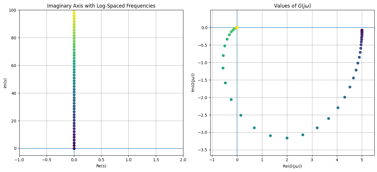
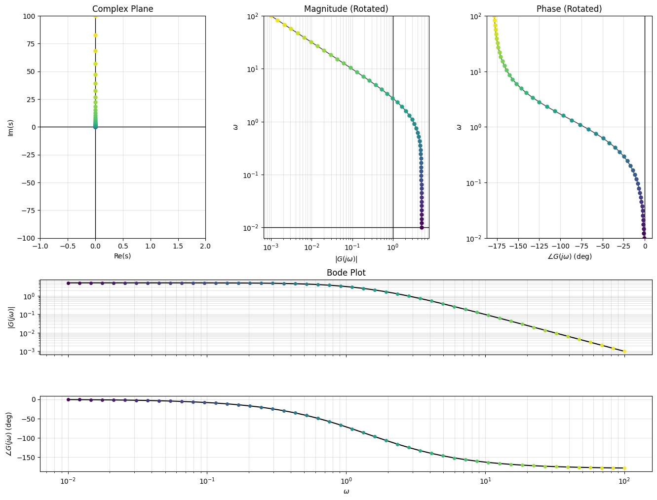
We will explore different graphical ways of visualizing this mapping. Initially, we will focus on what happens when \(s\) is restricted to the imaginary axis,

\[ s = j\omega, \quad \omega \in \mathbb{R}. \]

Once Loop Reflect

Loop transfer function and closed-loop stability

So far, we have focused on understanding how a transfer function \(G(s)\) maps complex inputs \(s\) to complex outputs \(G(s)\), and how this mapping can be visualized in different ways. However, in most applications, we are not interested in a system in isolation. Instead, systems are typically used in feedback configurations, where the output is fed back and compared to a reference. Consider a standard feedback system with plant \(P(s)\) and controller \(C(s)\).

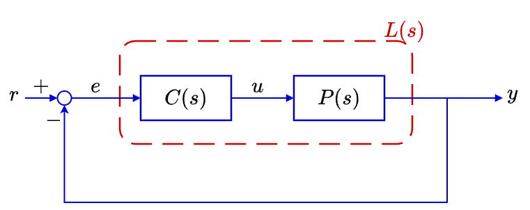
The closed-loop transfer function from \(r\) to \(y\) in the above configuration is

\[ T(s) = \frac{C(s)P(s)}{1 + C(s)P(s)}. \]

Define the loop transfer function

\[ L(s) = C(s)P(s). \]

Then

\[ T(s) = \frac{L(s)}{1 + L(s)}. \]

Closed-loop poles are determined by

\[ 1 + L(s) = 0. \]

Equivalently,

\[ L(s) = -1. \]

The condition \(L(s) = -1\) is critical for closed-loop stability.

Instead of analyzing \(T(s)\) directly, we can study \(L(s)\): When does \(L(s)\) reach the point \(-1\) in the complex plane?

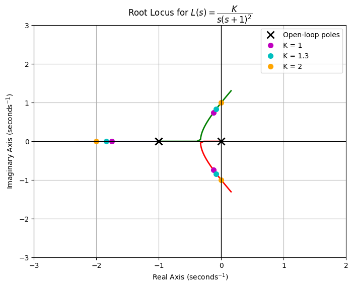
Take a closer look at the loop transfer function:

\[ L(s) = K \cdot \frac{1}{s(s+1)^2} \]

at \(K = 2\) and \(s = j\),

\[ L(j\omega) = 2 \cdot \frac{1}{j(j+1)^2} = -1 \]

When \(L = -1\) (i.e., for \(K = 2\) and \(\omega = 1\)), the closed-loop system becomes marginally stable.

Nyquist plots

The graphical representations of L(s) are powerful for analyzing the closed-loop stability (and other critical features). As will see, closed-loop stability is determined by how the curve \(L(j\omega)\) is positioned relative to the point \(-1\) in the complex plane.

To fully exploit this idea, we will extend our view beyond just the positive imaginary axis and consider a contour in the complex plane. This leads to the Nyquist plot, which provides a graphical tool for assessing closed-loop stability directly from the loop transfer function.

Nyquist plots build on so-called Nyquist contours. The Nyquist plot of a transfer function \(L\) is obtained by mapping a closed contour in the complex \(s\)-plane through the function \(L(s)\).

What is a Nyquist contour?

A Nyquist contour is a closed path in the complex plane that:

• encloses the right half-plane,

• is traversed clockwise,

• avoids poles of \(L(s)\) that lie on the imaginary axis.

The contour consists of three parts:

The imaginary axis segment

\[ s = j\omega, \quad \omega: -\infty \to +\infty \]

The indentations around imaginary-axis poles

• If \(L(s)\) has poles on the imaginary axis, we detour around them using small semicircles in the right half-plane.

• These have radius \(r\), and we take \(r \to 0.\)

A large semicircle at infinity

• A semicircle of radius \(R\) in the right half-plane: \(|s| = R, \quad R \to \infty.\)

Each point \(s\) on the contour is mapped through:

\[ s \;\longmapsto\; L(s). \]

This produces a curve in the complex \(L\)-plane called the Nyquist plot.

If \(L(s)\) has real coefficients, then:

\[ L(-j\omega) = \overline{L(j\omega)}. \]

So the Nyquist plot is symmetric about the real axis.

Walk through the derivation of the key aspects on an example

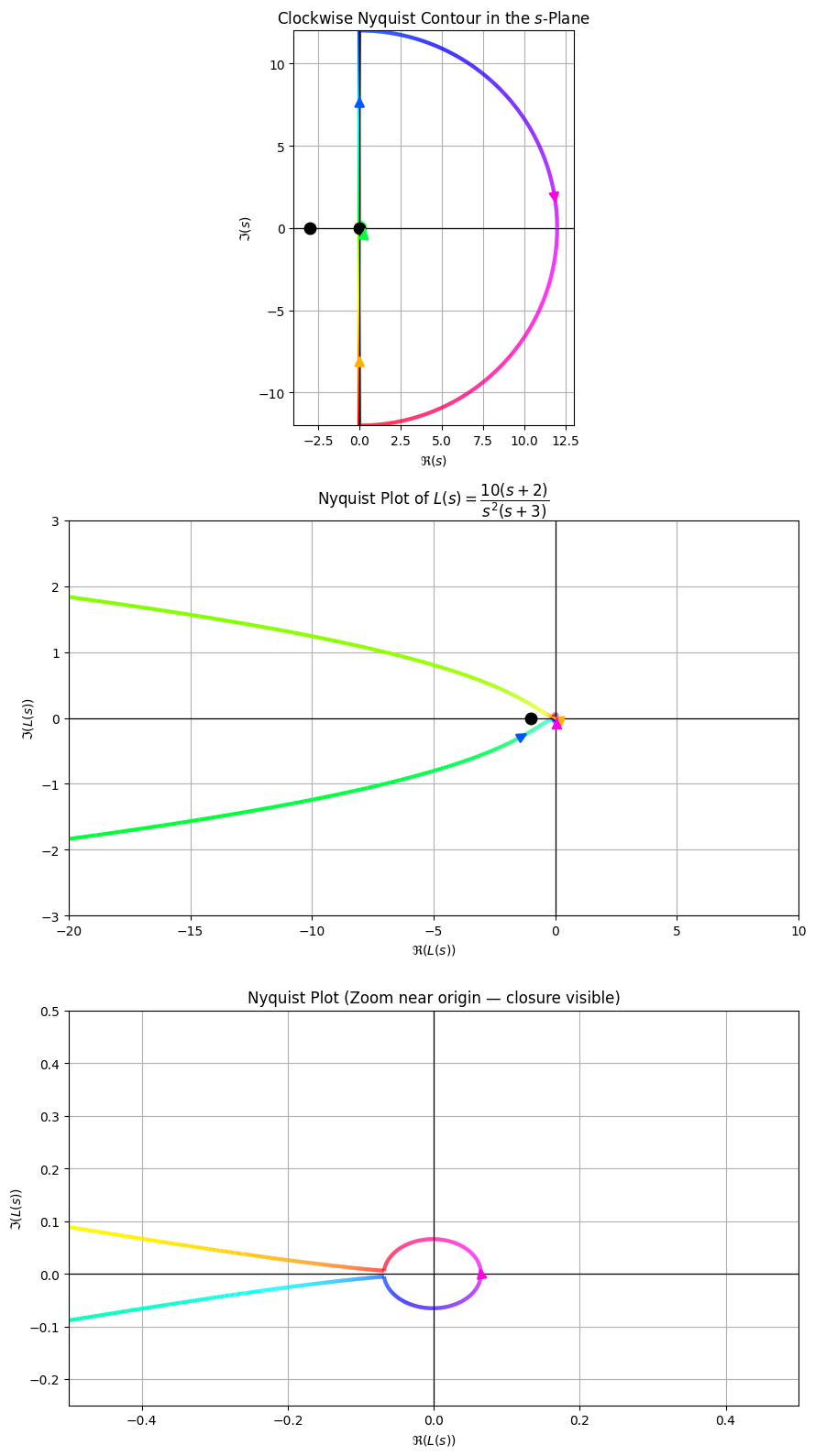
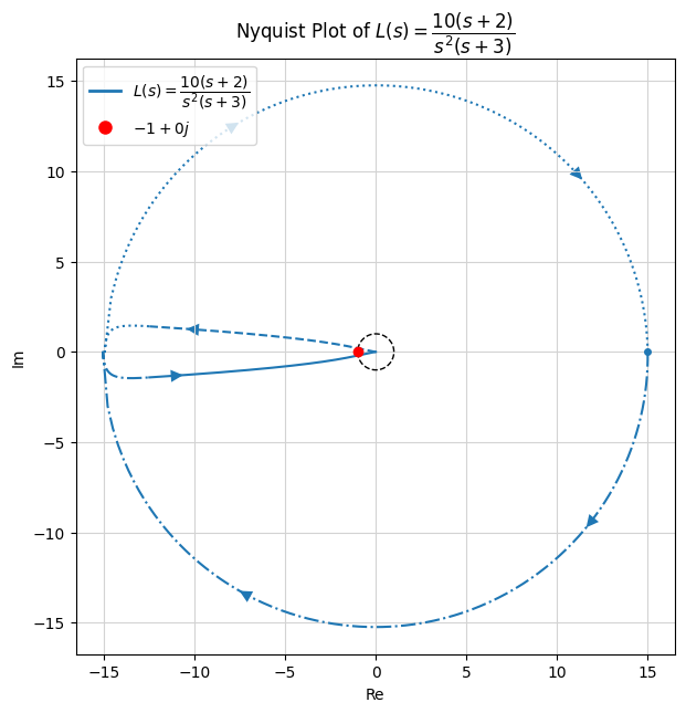
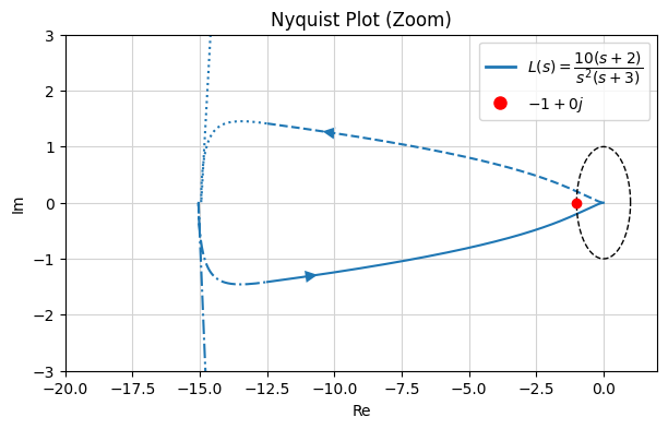
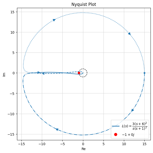
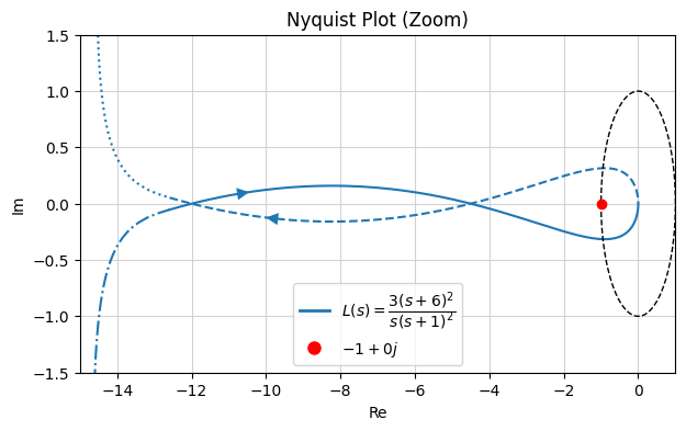
The loop transfer function is

\[ L(s) = \frac{10(s+2)}{s^2(s+3)} \]

with a zero as \(s = -2\) and three poles at \(s = 0\) (double pole) and \(s = -3.\)

The Nyquist contour is shown in the figure above: It follows the imaginary axis, detours around the origin into the right half-plane, and includes the large semicircle at infinity. It is traversed clockwise.

Behavior at infinity: As \(|s| \to \infty\),

\[ L(s) \approx \frac{10s}{s^3} = \frac{10}{s^2}. \]

Hence, magnitude \(\to 0\) and phase \(\to -2\angle s\).

The large semicircle in the \(s\)-plane maps to a small curve near the origin in the Nyquist plot.

Behavior near the origin: Near \(s = 0\),

\[ L(s) \approx\frac{10 \cdot 2}{3 s^2} = \frac{20}{3 s^2}. \]

Let

\[ s = \varepsilon e^{j\theta}. \]

Then

\[ L(s) \approx \frac{20}{3 \varepsilon^2} e^{-j 2\theta}. \]

Therefore, magnitude \(\to \infty\) and the angle rotates at twice the rate and in the opposite direction. The small detour around the origin maps to a large arc far away in the Nyquist plot.

Behavior along the imaginary axis: Set \(s = j\omega\):

\[ L(j\omega) = \frac{10(j\omega + 2)}{(j\omega)^2 (j\omega + 3)} = \frac{10(j\omega + 2)}{-\omega^2 (j\omega + 3)}. \]

This determines the main branches of the Nyquist plot.

Symmetry: Since the system has real coefficients, the Nyquist plot is symmetric about the real axis.

Nyquist stability criterion

• \(M_{ol}\): number of poles of the loop transfer function \(L(s)\) in the region enclosed by the Nyquist contour (i.e., poles of \(L(s)\) in the right half-plane)

• \(N\): number of clockwise encirclements of the point \(-1\) by the Nyquist plot

• \(M_{cl}\): number of closed-loop poles in the right half-plane

\[\boxed{ M_{cl} = M_{ol} + N} \]

Stability criterion: The closed-loop system is stable if and only if

\[ M_{cl} = 0. \]

Equivalently,

\[ M_{ol} + N = 0. \]

Special case: If \(L(s)\) has no right-half-plane poles (\(M_{ol} = 0\)), then the system is stable if and only if \( N = 0,\) i.e., the Nyquist plot does not encircle \(-1\).

Example: Nyquist stability for an inverted pendulum

Consider the loop transfer function (which is obtained using a simple model for an inverted pendulum and a derivative control)

\[ L(s) = \frac{k(s+2)}{s^2 - 1}. \]

For the analysis, we set \(k = 1.\)

The poles of \(L(s)\) are

\[ s = \pm 1, \]

and there is one pole in the right half-plane, namely at \(s=1\). Therefore,

\[ M_{ol} = 1. \]

With clockwise encirclements taken as positive,

\[ N = -1. \]

Consequently,

\[ M_{cl} = M_{ol} + N = 1 + (-1) = 0. \]

The closed-loop system has no right-half-plane poles, and is therefore stable.

Closed-loop poles:
(-0.5000000000000001+0.8660254037844385j)
(-0.5000000000000001-0.8660254037844385j)

/usr/local/lib/python3.12/dist-packages/control/freqplot.py:1509: UserWarning: number of encirclements was a non-integer value; this can happen is contour is not closed, possibly based on a frequency range that does not include zero.
  warnings.warn(

Example 2: Nyquist stability

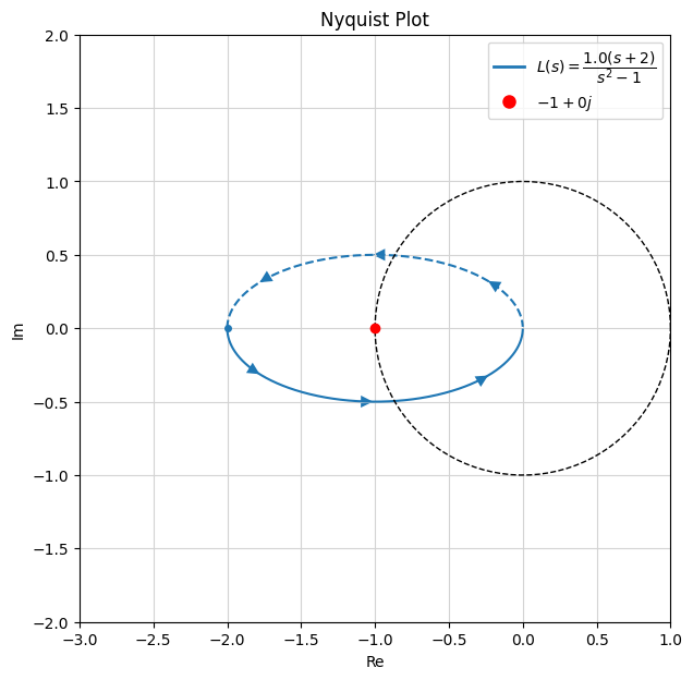
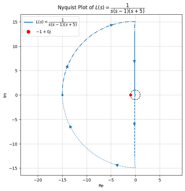
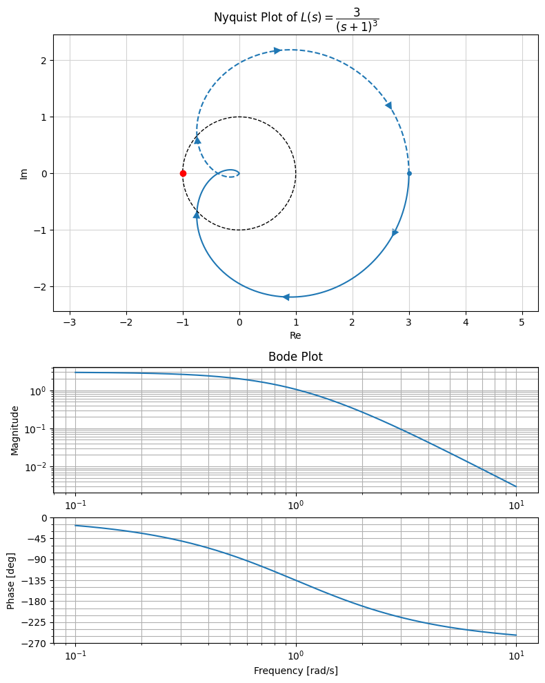
Consider the loop transfer function

\[ L(s) = \frac{k}{s(s-1)(s+5)}. \]

Since \(L(s)\) has a right-half-plane pole at \(s=1,\) and

\[ M_{ol}=1. \]

From the Nyquist plot, we observe one clockwise encirclement*of the point \(-1\). Therefore, \(N=1.\)

By the Nyquist criterion,

\[ M_{cl} = M_{ol} + N = 1 + 1 = 2. \]

So, the closed-loop system has two right-half-plane poles and is therefore unstable.

Example 3: Nyquist stability

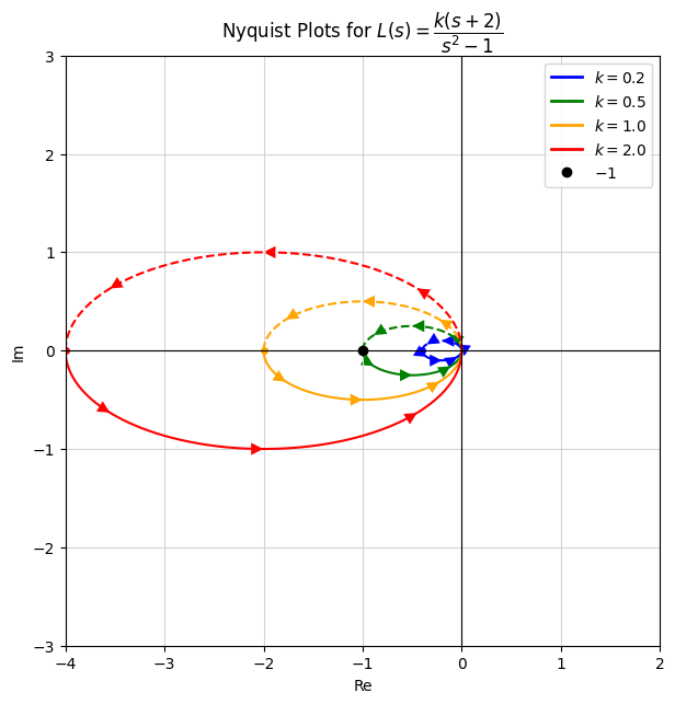
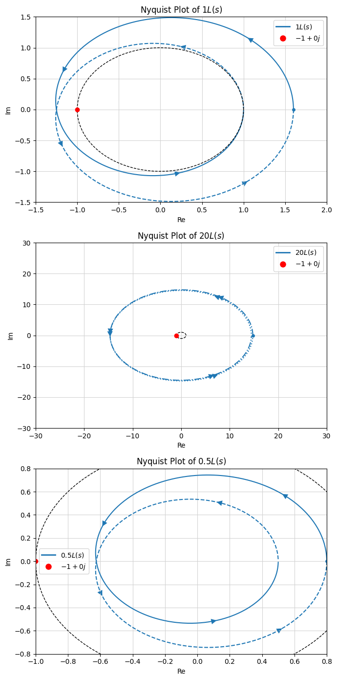
Consider the loop transfer function

\[ L(s)=\frac{s^2+10s+24}{s^2-8s+15}. \]

The poles of \(L(s)\) are

\[ s=3,\qquad s=5. \]

Both poles lie in the right half-plane. Therefore,

\[ M_{ol}=2. \]

Now consider the Nyquist plot of \(kL(s)\).

• For \(k=1\), the plot makes two counterclockwise encirclements of \(-1\): \(N=-2.\) Hence, $\( M_{cl}=M_{ol}+N=2-2=0, \)$ and the closed-loop system is stable.

• For \(k=20\), the plot still makes two counterclockwise encirclements of \(-1\): \( N=-2\). Therefore, M_{cl}=2-2=0$ and the closed-loop system is again stable.

• For \(k=0.5\), the plot does not encircle \(-1\): \(N=0.\) Therefore, $\( M_{cl}=2+0=2, \)$ and the closed-loop system is unstable.

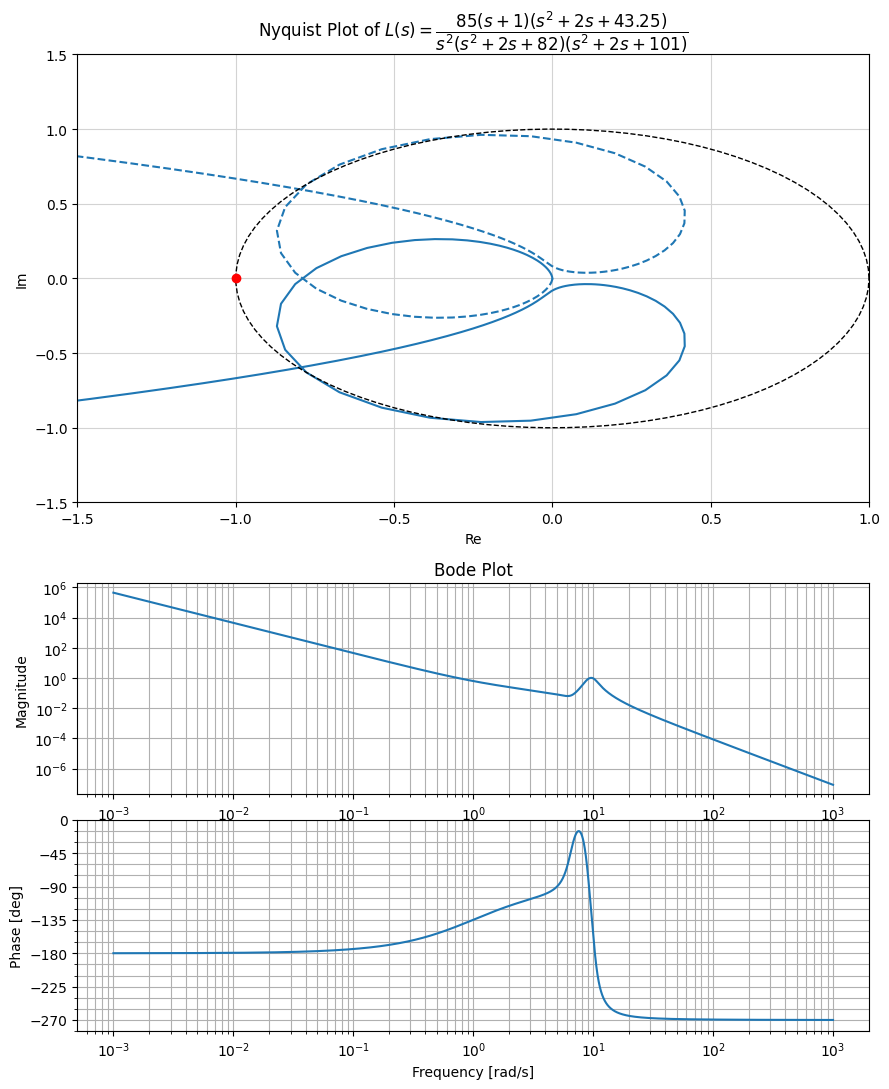
Example: Effect of gain on closed-loop stability using the Nyquist criterion

Consider the loop transfer function

\[ L(s)=k\,\frac{3(s+6)^2}{s(s+1)^2}. \]

Let

\[ L_0(s)=\frac{3(s+6)^2}{s(s+1)^2}, \qquad L(s)=kL_0(s). \]

The open-loop poles are at

\[ s=0,\qquad s=-1 \text{ (double)}. \]

Hence, there are no right-half-plane poles and

\[ M_{ol}=0. \]

To determine where stability changes, we find where the Nyquist plot crosses the real axis.

For \(s=j\omega\),

\[ L_0(j\omega)=\frac{3(j\omega+6)^2}{j\omega(j\omega+1)^2}. \]

The imaginary part is zero when

\[ \omega=2,\qquad \omega=3. \]

Evaluating the real part gives

\[ L_0(j2)=-12, \qquad L_0(j3)=-4.5. \]

Therefore, the real-axis crossings of \(L(s)=kL_0(s)\) occur at

\[ -12k \quad\text{and}\quad -4.5k. \]

The Nyquist plot passes through \(-1\) when

\[ -12k=-1 \quad\Rightarrow\quad k=\frac1{12}, \]

or

\[ -4.5k=-1 \quad\Rightarrow\quad k=\frac29. \]

Thus the gain has two critical values.

Since \(M_{ol}=0\), the Nyquist criterion gives

\[ M_{cl}=M_{ol}+N=N. \]

The stability of the closed-loop system varies for different ranges of \(k\):

• For $\( 0<k<\frac1{12}, \)\( the Nyquist plot does **not** encircle \)-1\(: \)\( N=0,\qquad M_{cl}=0. \)$ Therefore, the closed-loop system is stable.

• For $\( k=\frac1{12}, \)\( the Nyquist plot passes through \)-1$, so the closed-loop system is marginally stable.

• For $\( \frac1{12}<k<\frac29, \)\( the Nyquist plot has a nonzero net encirclement of \)-1\(: \)\( M_{cl}>0. \)$ Therefore, the closed-loop system is unstable.

• For $\( k=\frac29, \)\( the Nyquist plot again passes through \)-1$, so the closed-loop system is marginally stable.

• For $\( k>\frac29, \)\( the Nyquist plot does **not** encircle \)-1\(: \)\( N=0,\qquad M_{cl}=0. \)$ Therefore, the closed-loop system is stable.

Robustness margins

The Nyquist criterion provides a direct way to determine closed-loop stability from the open-loop transfer function \(L(s)\).

It also helps answer more refined questions such as:

• How robust is this stability to modeling uncertainty or perturbations?

These questions matter because a system can be stable in principle, yet still be fragile: small changes in gain, phase, or dynamics may drive it unstable.

To quantify this, we introduce robustness margins. We consider four key margins:

• Gain margin
  How much the loop gain can be increased before the system becomes unstable.

• Phase margin
  How much additional phase lag can be introduced before instability occurs.

• Time-delay margin
  The maximum time delay that can be tolerated before the system becomes unstable.

• Stability margin
  A geometric measure of how close the Nyquist plot comes to the critical point \(-1\).

Gain margin (\(g_m\))

The gain margin is the smallest factor by which the open-loop gain can be increased before the closed-loop system becomes unstable.

Consider a loop transfer function of the form

\[ k\,L(s), \]

with unity feedback.

We ask: How much can \(k\) be increased before instability occurs?

Define the phase crossover frequency \(\omega_{pc}\) as the frequency at which

\[ \angle L(j\omega_{pc}) = -180^\circ. \]

At \(\omega_{pc}\), the Nyquist plot lies on the negative real axis.

The gain margin is defined as

\[ g_m = \frac{1}{|L(j\omega_{pc})|}. \]

Phase margin (\(\varphi_m\))

The phase margin is the amount of additional phase lag required to bring the closed-loop system to the stability limit.

Consider a loop transfer function \(L(s)\) with unity feedback.

We ask: how much extra phase lag can be introduced before instability occurs?

Define the gain crossover frequency \(\omega_{gc}\) as the frequency at which

\[ |L(j\omega_{gc})| = 1. \]

At \(\omega_{gc}\), the Nyquist plot lies on the unit circle.

The phase margin is defined as

\[ \varphi_m = 180^\circ + \angle L(j\omega_{gc}). \]

Time-delay margin (\(T_m\))

The time-delay margin is the maximum time delay that can be introduced before the closed-loop system becomes unstable.

Consider a loop transfer function \(L(s)\) with unity feedback, and suppose a time delay \(T\) is introduced in the loop.

The transfer function of the delay block is

\[ e^{-Ts}. \]

The overall loop transfer function becomes

\[ e^{-Ts} L(s). \]

At frequency \(\omega\), the delay contributes

\[ e^{-j\omega T}, \]

which corresponds to a pure phase lag of \(-\omega T.\)

At the stability boundary, the Nyquist plot must pass through \(-1\):

\[ -1 = e^{-j\omega T} L(j\omega). \]

Let \(\omega_{gc}\) be the gain crossover frequency, defined by

\[ |L(j\omega_{gc})| = 1. \]

At this frequency, the Nyquist plot lies on the unit circle. At \(\omega_{gc}\), instability occurs when the additional phase lag due to delay equals the phase margin.

Thus,

\[ \omega_{gc} T_m = \varphi_m. \]

Hence, the time-delay margin is

\[ T_m = \frac{\varphi_m}{\omega_{gc}}. \]

Stability margin (\(s_m\))

The stability margin is the shortest distance from the Nyquist curve to the critical point \(-1\). It is defined as

\[ s_m = \min_{\omega} \; |\,L(j\omega) + 1\,|. \]

Margins from control.stability_margins:
  Gain margin gm        = 1.2624534993428793
  Gain margin (dB)      = [2.02430781]
  Phase margin pm       = 36.73682917236735 deg
  Stability margin sm   = 0.18720571399555436
  Phase crossover freq  = 10.343107968625196 rad/s
  Gain crossover freq   = 0.7436481751781284 rad/s
  Stability margin freq = 10.272733778234562 rad/s