All rights reserved. For enrolled students only. Redistribution prohibited.

Linear Systems

• General solution

• Matrix exponentials

• Free response

• Similarity transformation and diagonalization

• Stability

• Second-order systems

• Step response

Solution to a “general” linear system

Recall that the solution for a first-order (single-variable, i.e., scalar) linear system

\[ \dot{x}(t) = A x(t) + B u(t), \]

where \(A \in \mathbb{R}\) and \(B \in \mathbb{R}\) is given by

\[ x(t) = e^{A t} x_0 + \int_{0}^{t} e^{A (t - \tau)} B\,u(\tau)\,d\tau. \]

Let us now focus on a general case where \(A \in \mathbb{R}^{n\times x}\) and \(B \in \mathbb{R}^{n \times m}\) with \(n \geq 1\) and \(m \geq 1:\)

\[ \dot{x}(t) = A x(t) + B u(t). \]

That is, the state is an \(n\)-dimensional vector and the input is an \(m\)-dimensional vector.

What is the solution in this case? It takes exactly the same form:

\[ x(t) = e^{A t} x_0 + \int_{0}^{t} e^{A (t - \tau)} B\,u(\tau)\,d\tau. \]

But, what is \(e^{At}\) when \(A \in \mathbb{R}^{n \times n}\)?

Definition of matrix exponentials

For a definition of the matrix exponential \(e^{At}\) (for \(A \in \mathbb{R}^{n \times n}\)), recall the Taylor series expansion for the exponential function \(e^{at}\) (for \(a \in \mathbb{R}\)) around \(t = 0\):

\[ e^{a t} = 1 + a t + \frac{(a t)^2}{2!} + \frac{(a t)^3}{3!} + \cdots .\]

For \(A \in \mathbb{R}^{n\times n}\), the matrix function \(e^{A t}\) is defined by plugging the matrix \(A\) for \(a\) in the above series:

\[ e^{A t} = I + t A + \frac{t^2 A^2}{2!} + \frac{t^3 A^3}{3!} + \cdots .\]

Here \(A^k\) denotes the product of \(A\) with itself \(k\) times:

\[ A^k = A \cdot A \cdot \ldots \cdot A. \]

Verification of the solution to the general linear system

Given this definition of the matrix exponential, how do we know \(x(t) = e^{A t} x_0 + \int_{0}^{t} e^{A (t - \tau)} B\,u(\tau)\,d\tau\) is a solution to the general linear system \(\dot{x}(t) = A x(t) + B u(t)\) ? See this page.

How to compute the matrix exponential?

The infinite series above provide a means for computing \(A.\) We will see examples of such computation later. But, such computation can be tedious and sheds little light on the analysis of and design for linear systems. To gain such insight, let’s begin with some special cases where \(A\) is 2-by-2 (pay attention below whether the entries of the matrix are real- or complex-valued).

\[\begin{split} A_1 = \begin{bmatrix} \alpha_1 & 0 \\ 0 & \alpha_2 \end{bmatrix}, \quad \alpha_i \in \mathbb{C} \;\Longrightarrow\; e^{A_1t} = \begin{bmatrix} e^{\alpha_1 t} & 0 \\ 0 & e^{\alpha_2 t} \end{bmatrix}.\end{split}\]

\[\begin{split}A_2 = \begin{bmatrix} 0 & \beta \\ -\beta & 0 \end{bmatrix}, \quad \beta \in \mathbb{R} \;\Longrightarrow\; e^{A_2t} = \begin{bmatrix} \cos(\beta t) & \sin(\beta t) \\ -\sin(\beta t) & \cos(\beta t) \end{bmatrix}.\end{split}\]

\[\begin{split}A_3 = \begin{bmatrix} \alpha & \beta \\ -\beta & \alpha \end{bmatrix}, \quad \alpha,\beta \in \mathbb{R} \;\Longrightarrow\; e^{A_3t} = e^{\alpha t} \begin{bmatrix} \cos(\beta t) & \sin(\beta t) \\ -\sin(\beta t) & \cos(\beta t) \end{bmatrix}.\end{split}\]

How are the matrix exponential derived? Check this note for the cases above: Matrix Exponential Derivation

From matrix exponential to free response

Once the matrix exponential is computed, the free response (the part of the solution that evolves without the effect of an external input) from an initial condition \(x_0 \in \mathbb{R}^n\) can be computed as follows:

\[x(t) = e^{At} x_0\]

\[y(t) = Cx(t) = C e^{At} x_0.\]

Matrix exponential for a diagonal matrix

The first of the three special 2-by-2 matrices above was a diagonal matrix (with complex-valued diagonal entries). The form of the matrix exponential generalizes to n-by-n diagonal matrices with complex-valued diagonal entries.

\[\begin{split} A=\begin{bmatrix} \alpha_1 & 0 & \cdots & 0\\ 0 & \alpha_2 & \cdots & 0\\ \vdots & \vdots & \ddots & \vdots\\ 0 & 0 & \cdots & \alpha_n \end{bmatrix} \;\Longrightarrow\; e^{At}=\begin{bmatrix} e^{\alpha_1 t} & 0 & \cdots & 0\\ 0 & e^{\alpha_2 t} & \cdots & 0\\ \vdots & \vdots & \ddots & \vdots\\ 0 & 0 & \cdots & e^{\alpha_n t} \end{bmatrix}. \end{split}\]

Observe that for this special matrix, the matrix exponential is very straightforward. Can we make use of this fact in computing the matrix exponential of a generic matrix? Before seeing for what kind of matrices we can leverage this observation, let’s first look into how.

Similarity transformations

Fact from linear algebra: Two n-by-n matrices \(A\) and \(\widetilde{A}\) are called similar if there exists an invertible n-by-n matrix \(P\) such that

\[\widetilde{A} = P^{-1} A P\]

or equivalently

\[P \widetilde{A} P^{-1} = A. \]

For \(A \in \mathbb{C}^{n \times n}\) and \(P \in \mathbb{C}^{n \times n}\) invertible, the following holds.

\[\begin{split} \begin{aligned} e^{A t} &= I + tA + \frac{t^2 A^2}{2!} + \frac{t^3 A^3}{3!} + \cdots \\[6pt] &= P I P^{-1} + t\, \widetilde{A} + \frac{t^2 P \widetilde{A}^2 P^{-1}}{2!} + \frac{t^3 P \widetilde{A}^3 P^{-1}}{3!} + \cdots \\[6pt] &= P \left( I + t \widetilde{A} + \frac{t^2 \widetilde{A}^2}{2!} + \frac{t^3 \widetilde{A}^3}{3!} + \cdots \right) P^{-1} \\[6pt] &= P\, e^{\widetilde{A}\, t}\, P^{-1} \\[6pt] \end{aligned} \end{split}\]

(In this derivation, we used the fact that \((P^{-1} A P)^k = P^{-1} A^k P\) for \(k = 1,2,\dots\) and \(I = P^{-1} I P\).)

Let’s re-write the end-to-end result:

\[ e^{A t} = P\, e^{\widetilde{A}\, t}\, P^{-1}.\]

Now, the question is “what if computing \(e^{\widetilde{A}\, t}\) is easy even if it is not easy for \(e^{A t}\)”? For example, what if \(\tilde A\) is a diagonal matrix? Then, we can compute \(e^{A t}\) in two steps:

1. First, compute \(e^{\widetilde{A}\, t}\) (it is given above).

2. Then, muptiply the result by \(P\) (from the left) and \(P^{-1}\) (from the right): \(P\, e^{\widetilde{A}\, t}\, P^{-1}\) to obtain \(e^{A t}\).

Here is a small example:

\[\begin{split} A = \begin{bmatrix} 0 & 1 \\ -2 & -3 \end{bmatrix}, \qquad \dot{x} = A x,\quad x(0)=x_0. \end{split}\]

\(A\) is not in any of the special forms we’ve seen. Let \(P\) be

\[\begin{split} P = \begin{bmatrix} -1 & -1 \\ 2 & 1 \end{bmatrix} \end{split}\]

Then

\[\begin{split} \widetilde{A} = P^{-1} A P = \begin{bmatrix} -2 & 0 \\ 0 & -1 \end{bmatrix} \end{split}\]

which is diagonal.

Let’s apply the two steps:

\[\begin{split} e^{\widetilde{A}t} = \begin{bmatrix} e^{-2 t} & 0 \\ 0 & e^{-t} \end{bmatrix}\end{split}\]

and

\[\begin{split} \begin{aligned} e^{A t} &= P\, e^{\widetilde A t}\, P^{-1} \\[6pt] &= \begin{bmatrix} -1 & -1\\ \;\,2 & \;\,1 \end{bmatrix} \begin{bmatrix} e^{-2t} & 0\\ 0 & e^{-t} \end{bmatrix} \begin{bmatrix} -1 & -1\\ \;\,2 & \;\,1 \end{bmatrix}^{-1} \\[10pt] &= \begin{bmatrix} - e^{-2t} + 2 e^{-t} & - e^{-2t} + e^{-t} \\[4pt] \;\,2 e^{-2t} - 2 e^{-t} & \;\,2 e^{-2t} - e^{-t} \end{bmatrix}. \end{aligned} \end{split}\]

Diagonalization

The next question is, for a matrix \(A,\) when a similarity transformation \(P\) exists such that \(\widetilde{A} = P^{-1} A P\) is diagonal.

One sufficient condition is the following: When the eigenvalues of \(A\) are distinct, then there exists a similarity transformation \(P\) such that \(\widetilde{A} = P^{-1} A P\) is diagonal.

Let \(\lambda_1, \ldots, \lambda_n\) be the eigenvalues of A, and let \(\lambda_1, \ldots, \lambda_n\) be the corresponding eigenvalues. Note that both eigenvalues and eigenvectors can be complex-valued (even when \(A\) is real-valued). Assume that \(\lambda_1, \ldots, \lambda_n\) are distinct. Then, \(\lambda_1, \ldots, \lambda_n\) are linearly independent. And, the similarity transformation \(P\) can be constructed as

\[\begin{split} P = \begin{bmatrix} \vert & \vert & & \vert \\ v_1 & v_2 & \cdots & v_n \\ \vert & \vert & & \vert \end{bmatrix}. \end{split}\]

Then,

\[\Lambda = P^{-1} A P\]

is diagonal (consider \(\Lambda\) as \(\widetilde{A}\) above) where

\[\begin{split} \Lambda = \begin{bmatrix} \lambda_1 & 0 & \cdots & 0 \\ 0 & \lambda_2 & \cdots & 0 \\ \vdots & \vdots & \ddots & \vdots \\ 0 & 0 & \cdots & \lambda_n \end{bmatrix}. \end{split}\]

Let’s look at an example.

\[\begin{split} A= \begin{bmatrix} 7 & 0 & 5 & -5\\ 18 & 2 & 16 & -10\\ -8 & 0 & -7 & 6\\ 0 & 0 & -2 & 1 \end{bmatrix}. \end{split}\]

The eigenvalues:

\[ \lambda_1=2,\qquad \lambda_2=-1,\qquad \lambda_3=1+2i,\qquad \lambda_4=1-2i. \]

The eigenvactors form the the similarity transformation:

\[\begin{split} P= \begin{bmatrix} 0 & 0 & 1+2j & 1-2j\\ -2 & -2 & 2 & 2\\ 0 & 1 & -2j & 2j\\ 0 & 1 & 2 & 2 \end{bmatrix}\end{split}\]

Diagonalization \( \Lambda = P^{-1} A P\):

\[\begin{split} \Lambda = \begin{bmatrix} 2 & 0 & 0 & 0\\ 0 & -1 & 0 & 0\\ 0 & 0 & 1+2j & 0\\ 0 & 0 & 0 & 1-2j \end{bmatrix}, \end{split}\]

Refresh your memory about the computation of eigenvalues and eigenvectors here.

A =
 [[  7.   0.   5.  -5.]
 [ 18.   2.  16. -10.]
 [ -8.   0.  -7.   6.]
 [  0.   0.  -2.   1.]]

Eigenvalues =
 [ 2.+0.j  1.+2.j  1.-2.j -1.+0.j]

P (eigenvectors as columns) =
 [[ 0.      +0.j        0.542326+0.j        0.542326-0.j
   0.      +0.j      ]
 [ 1.      +0.j        0.21693 -0.433861j  0.21693 +0.433861j
   0.816497+0.j      ]
 [ 0.      +0.j       -0.433861-0.21693j  -0.433861+0.21693j
  -0.408248+0.j      ]
 [ 0.      +0.j        0.21693 -0.433861j  0.21693 +0.433861j
  -0.408248+0.j      ]]

Lambda = P^{-1} A P =
 [[ 2.+0.j -0.-0.j -0.+0.j -0.+0.j]
 [ 0.+0.j  1.+2.j  0.+0.j -0.+0.j]
 [ 0.+0.j -0.-0.j  1.-2.j -0.-0.j]
 [ 0.+0.j  0.+0.j  0.+0.j -1.-0.j]]

||A P - P Lambda||_F = 3.193462903526722e-15
||Lambda - diag(eigvals)||_F = 1.0595244504700326e-14

Effect of diagonalization

A similarity transformation corresponds to a change of coordinates between state variables.
If we define new coordinates \(\widetilde{x}\) by

\[x = P\,\widetilde{x},\]

then solutions of the diagonal system

\[\dot{\widetilde x} = \widetilde{A} \widetilde{x}\]

map directly to solutions of the original system \(\dot x = A x\).
Diagonalization shows that the apparent coupling in the original system comes from the coordinate transformation \(P\), not from additional dynamics.

The example below dmeonstrates this observation (using a 2-by-2 matrix and a similarity transformation we introduced earlier).

Stability

Because similarity transformations only change coordinates and not the underlying dynamics, long-term properties of the system, such as stability and asymptotic behavior, can be determined directly from the diagonalized system.

Let’s focus on the free responses of the system.

\[x(t)=e^{At}x_0 = P e^{\Lambda t} P^{-1}\]

where only \(e^{\Lambda t}\) is the only term that changes with time. The matrices \(P\) and \(P^{-1}\) are constant matrices. Let’s take a closer look at \(e^{\Lambda t}\):

\[\begin{split} \begin{bmatrix} e^{\lambda_1 t} & 0 & \cdots & 0\\ 0 & e^{\lambda_2 t} & \cdots & 0\\ \vdots & \vdots & \ddots & \vdots\\ 0 & 0 & \cdots & e^{\lambda_n t} \end{bmatrix}. \end{split}\]

Here, \(\lambda_1,\ldots,\lambda_n\) are the eigenvalues of \(A\) and they can be real- or complex-valued.

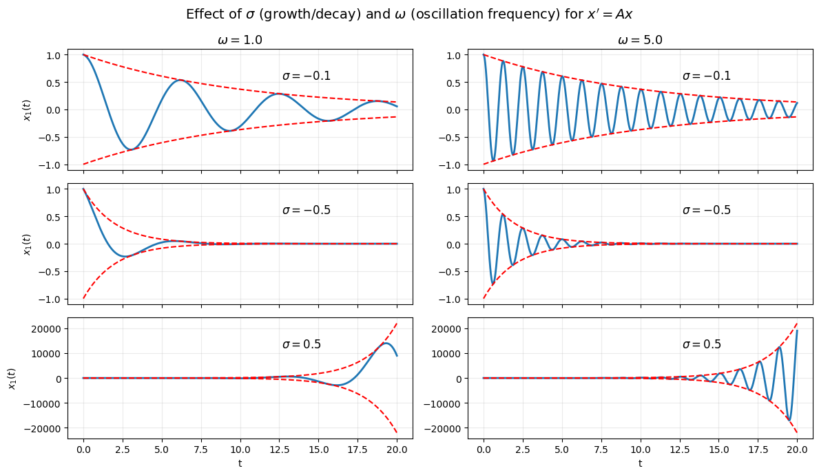
• Real-valued eigenvalue \(\lambda\):

\[\begin{split} e^{\lambda t}\;\longrightarrow\; \begin{cases} 0, & \text{if } \lambda < 0,\\[6pt] 1, & \text{if } \lambda = 0,\\[6pt] \infty, & \text{if } \lambda > 0, \end{cases} \qquad \text{as } t \to \infty. \end{split}\]

• To understand the case with complex-valued eigenvalue \(\lambda\), let’s recall a few facts.

  • If \(\lambda = \lambda_{real} + j \lambda_{imaginary}\) is an eigenvalue, then its complex conjugate \(\lambda_{real} - j \lambda_{imaginary}\) must also be a egeinvalue. (Let’s abbreviate the notation: \(\lambda = \lambda_{r} + j \lambda_{i}\).)
    

  • Making use of the Euler’s formula:
    

  \[ e^{\lambda t} = e^{(\lambda_{r} + j \lambda_{i}) t} = e^{\lambda_{r}t} e^{j \lambda_{i} t} = e^{\lambda_{r}t} (cos (\lambda_it)+j sin(\lambda_i t)).\]

  Then,
  

  \[\begin{split} e^{\lambda t} \;\longrightarrow\; \begin{cases} 0, & \text{if } \operatorname{Re}\lambda < 0,\\[6pt] \text{bounded (oscillatory)}, & \text{if } \operatorname{Re}\lambda = 0,\\[6pt] \infty, & \text{if } \operatorname{Re}\lambda > 0, \end{cases} \qquad \text{as } t \to \infty. \end{split}\]

An important outcome: A necessary and sufficient conditions for the stability of a linear system.

• A linear system is stable if and only if,

  \[\operatorname{Re}\lambda < 0\]

  for all eigenvalues \(\lambda\) of \(A\).

• The system is unstable if and only if,

  \[\operatorname{Re}\lambda > 0\]

  for some eigenvalue \(\lambda\) of \(A\). (This sentence may be deceptively simple. Make sure that you understand what that means.)

• The system is marginally stable if and only if, for all eigenvalues \(\lambda\) of \(A\),

  \[\operatorname{Re}\lambda \leq 0\]

  and for some eigenvalue \(\lambda\) of \(A\),

  \[\operatorname{Re}\lambda = 0.\]

Note that these statements are derived under the assumption that \(A\) has distinct eigenvalues. If \(A\) has repeated eigenvalues, the definition for the stable case remains the same. However, the definitions for the other cases change. We will revise these definitions later to capture the case where \(A\) has repeated eigenvalues.

What do these terms mean in terms of the system behavior?

Recall that for the first-order systems, we connected these definitions to the initial conditions and asymptotic behavior. Analogous definitions hold for the general case:

• The system is stable if and only if the free response converges to the origin for all initial conditions.

• The system is unstable if and only if the magnitude of the free response diverges to infinity for some initial condition.

• The system is marginally stable if and only if the magnitude of the free response is bounded for all initial conditions, and the free response does not converge to the origin for some initial condition.

Essentially, decay corresponds to stability, bounded (oscillatory) behavior corresponds to marginal stability, and growth corresponds to instability.

Block diagonalization

Can we always diagonalize the \(A\) matrix? We may not be able to diagonalize fully, but we can get very close.

Let \(A \in \mathbb{R}^{n \times n}\).
There exists an invertible matrix \(P\) such that \(P^{-1} A P = J\), where

\[\begin{split} J = \begin{bmatrix} J_1 & 0 & \cdots & 0 \\ 0 & J_2 & \cdots & 0 \\ \vdots & \vdots & \ddots & \vdots \\ 0 & 0 & \cdots & J_p \end{bmatrix}, \end{split}\]

and

\[\begin{split} J_i = \begin{bmatrix} \lambda_i & 1 & 0 & \cdots & 0 \\ 0 & \lambda_i & 1 & \cdots & 0 \\ \vdots & \vdots & \vdots & \ddots & 1 \\ 0 & 0 & 0 & \cdots & \lambda_i \end{bmatrix}\in\mathbb{C}^{n_i\times n_i} \end{split}\]

and \(n_i\) is the algebraic multiplicity of eigenvalue \(\lambda_i\).

When all eigenvalues are distinct, then \(n_i = \) for all eigenvalues and full diagonalization is possible.

It is straightforward to derive the matrix exponential for \(J\) in terms of the matrix exponential of the diagonal blocks \(J_1,\ldots, J_p\):

\[\begin{split} e^{J t} = \begin{bmatrix} e^{J_1 t} & 0 & \cdots & 0 \\ 0 & e^{J_2 t} & \cdots & 0 \\ \vdots & \vdots & \ddots & \vdots \\ 0 & 0 & \cdots & e^{J_t t} \end{bmatrix}. \end{split}\]

And, \(e^{J_i t}\) has the structure (see Matrix Exponential Derivation: Special Case):

\[\begin{split} e^{J_i t} = \begin{bmatrix} e^{\lambda_i t} & t e^{\lambda_i t} & {t^2 e^{\lambda_i t}}/{2!} & \cdots & {t^{n_i-1} e^{\lambda_i t}}/{(n-1)!} \\ 0 & e^{\lambda_i t} & t e^{\lambda_i t} & \cdots & {t^{n_i-2} e^{\lambda_i t}}/{(n_i-2)!} \\ \vdots & \vdots & \ddots & \ddots & \vdots \\ 0 & 0 & \cdots & e^{\lambda_i t} & t e^{\lambda_i t} \\ 0 & 0 & \cdots & 0 & e^{\lambda_i t} \end{bmatrix}. \end{split}\]

The entries involve terms of the form

\[ t^k e^{\lambda_i t}, \qquad k = 0,1,2,3,\dots. \]

Simulation below allows you to explore these functions for different values of \(\lambda\).

Although polynomial factors such as \(t^k\) can cause significant transient growth in the solutions, the long-term behavior is still governed by the exponential term \(e^{\lambda t}\). When \(\operatorname{Re}(\lambda) < 0\), the exponential decay dominates any polynomial growth, and all solutions decay to zero as \(t \to \infty\).

As a result, the presence of repeated eigenvalues or non-diagonalizable dynamics does not change the stability classification of the system. Stability depends only on the real parts of the eigenvalues, not on the polynomial factors that appear in the solution.

Stability for systems with repeated eigenvalues

If the \(A\) matrix has repeated eigenvalues, the stability definitions using the eigenvalues change depending on the shape of the \(J\) matrix and whether these repeated eigenvalues are on the imaginary axis.

• A linear system is stable if and only if

  \[\operatorname{Re}\lambda < 0\]

  for all eigenvalues \(\lambda\) of \(A\).

• The system is unstable if and only if, for some eigenvalue \(\lambda\) of \(A\),

  \[\operatorname{Re}\lambda > 0,\]

  or for some eigenvalue \(\lambda\) that has a Jordan block of size strictly greater than 1

  \[\operatorname{Re}\lambda = 0.\]

• The system is marginally stable if and only if, for all eigenvalues \(\lambda\) of \(A\),

  \[\operatorname{Re}\lambda \leq 0,\]

  and the Jordan block size is 1 for all eigenvalues \(\lambda\) of \(A\) such that

  \[\operatorname{Re}\lambda = 0.\]

For example, a system with

\[\begin{split}A=\begin{bmatrix} 0 & 1\\ 0 & 0\\ \end{bmatrix},\end{split}\]

which has a repeated eigenvalue at \(0\). Since the the corresponding Jordan block has size \(2\), the system is unstable. Note that the unstability is due to the growing \(te^{0t}\) term in the free response.

Consider a system with

\[\begin{split}A=\begin{bmatrix} 0 & 0\\ 0 & 0\\ \end{bmatrix},\end{split}\]

which has a repeated eigenvalue at \(0\). Since the corresponding Jordan blocks have size \(1\), the system is marginally stable. In fact, \(\dot{x} = [0,0]^{\top}\), meaning that the system remains at its initial condition.

Modes of a linear system

(The following observation generalizes to the case when \(A\) cannot be fully diagonalized but let us consider the case in which it can be for clarity.)

Recall that

\[\begin{split} x(t) = e^{A t} x_0 = P\, e^{\Lambda\, t}\, P^{-1}x_0 = P\, \begin{bmatrix} e^{\lambda_1 t} & 0 & \cdots & 0\\ 0 & e^{\lambda_2 t} & \cdots & 0\\ \vdots & \vdots & \ddots & \vdots\\ 0 & 0 & \cdots & e^{\lambda_n t} \end{bmatrix} \, P^{-1}x_0.\end{split}\]

The free response is a linear combination of the functions \(e^{\lambda_1 t}, \ldots, e^{\lambda_n t}.\) (Note that some of the eigenvalues may be complex along with their complex congugates. We will develop a cleaner interpretation of that case later. For now, let’s proceed with potentially complex entries in the diagonal matrix exponential.)

We refer to \(e^{\lambda_1 t}, \ldots, e^{\lambda_n t}\) as the modes of the system.

We will look into an example on how the modes of a linear system determine the free response of a linear system. It may be useful to recall that the columns of the transformation \(P\) are the eigenvectors of \(A\):

\[\begin{split} P = \begin{bmatrix} \vert & \vert & & \vert \\ v_1 & v_2 & \cdots & v_n \\ \vert & \vert & & \vert \end{bmatrix}, \end{split}\]

and any initial condition \(x_0\) can be written as a linear combination of \(v_1,\ldots, v_n\).

Note that \(A\) is fully-diagonalizable and, therefore, \(v_1,\ldots, v_n\) are linearly independent. It implies that the coefficients of the linear combination are unique. Let

\[x_{0} = \sum_{i=1}^{n} c_{i} v_{i} = Pc\]

where \(c = [c_{1}, \ldots, c_{n}]^{\top}\) is the vector of coefficients. This implies \(c = P^{-1}x_{0}\). Recall that

\[x(t) = P e^{Λ t} P^{-1} x_{0}.\]

Substituting \(c = P^{-1}x_{0}\), we get

\[x(t) = P e^{Λ t} c.\]

After some matrix algebra, \(x(t)\) can be represented as

\[x(t) = \sum_{i=1}^{n} c_{i} v_{i} e^{\lambda_{i}t}.\]

The free response is a superposition of eigenmodes, each scaled by how strongly the initial condition projects onto its eigenvector and evolving according to the associated eigenvalue.

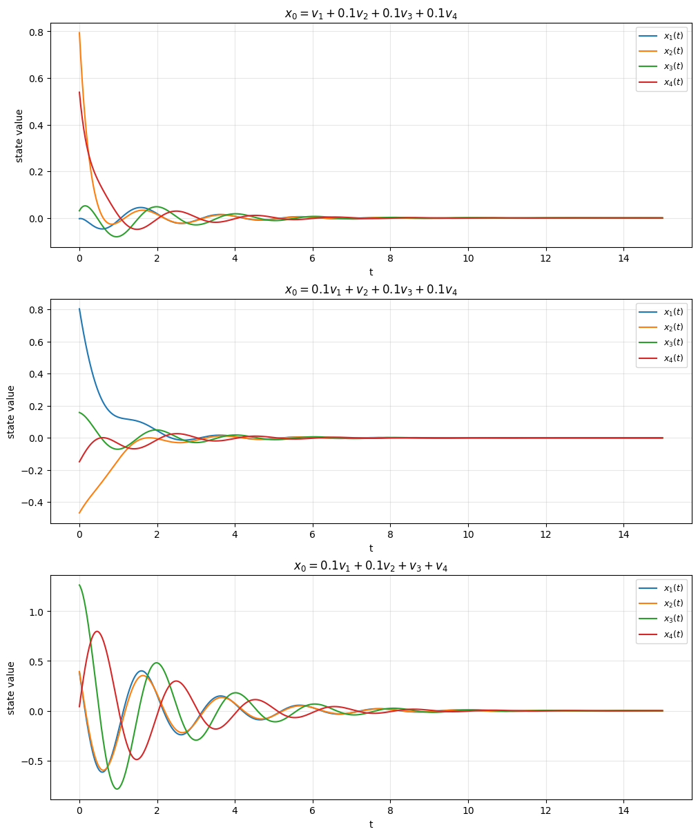
What is the implication? The free response of the system depends on the coefficients of the modes. For example, if the initial state has no components in the subspace spanned by the complex eigenvalues (\(c_{i} = 0\) for all \(λ_{i}\) such that \(\text{Im}(λ_{i}) \neq 0\)), then the free response does not oscillate. More importantly, the convergence of the free response depends on the initial state. If, the initial state

• has a component in the subspace spanned by the unstable modes (\(c_{i} \neq 0\) for some \(λ_{i}\) such that \(\text{Re}(λ_{i})>0\)), then the free response diverges,

• has no component in the subspace spanned by the unstable and marginally stable modes (\(c_{i} = 0\) for all \(λ_{i}\) such that \(\text{Re}(λ_{i})\geq 0\)), then the free response converges to 0.

Remark on stability vs. convergence of a particular initial state: The above discussion describes the convergence behavior from a particular initial state, whereas stability is a system-level property that concerns all initial states. Remember that stability can be verified by checking only the eigenvalues.

We may have a system that is not stable (\(\text{Re}(\lambda_{i}) \geq 0\) for some \(λ_{i}\)), but the free response converges to \(0\) for some initial condition.

Note that we did not encounter such cases for first-order systems since there is only one eigenvalue (the scalar \(A\)) and one eigenvector (any non-zero reel number, e.g., \(1\)). For an unstable first-order system (\(A > 0\)), the subspace spanned by the unstable mode is \(\mathbb{R}\), and all non-zero initial conditions lie in this space. Consequently, all non-zero initial conditions diverge.

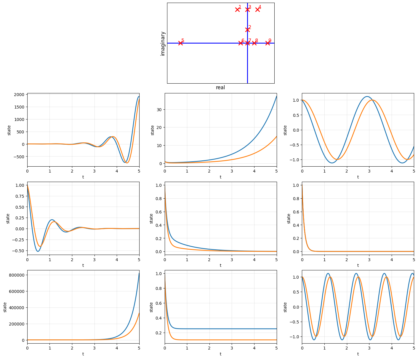
Eigenvalues:
[-3.79408178+0.j         -1.64231316+0.j         -0.48180253+3.08840707j
 -0.48180253-3.08840707j]

A closer look at second-order systems

It is worth taking a closer look into second-order systems for intuition:

\[ \dot{x} = A x, \qquad A \in \mathbb{R}^{2 \times 2}. \]

By now, we have established that the eigenvalues of \(A\) play a central role. For \(A \in \mathbb{R}^{2 \times 2}\), there are several possibilities:

1. Real and distinct eigenvalues: \(\lambda_1\) and \(\lambda_2\). In this case, \(A\) can be diagonalized to

\[\begin{split}\begin{bmatrix} \lambda_1 & 0 \\ 0 & \lambda_2 \end{bmatrix}.\end{split}\]

2. Complex eigenvalues, \(\lambda\) and \(\lambda^*\), since complex eigenvalues come in complex conjugate pairs.

3. Repeated eigenvalues, \(\lambda\) and \(\lambda\), which have to real since they are same. In this case, there are two possibilities.

   • \(A\) can be fully diagonalized, which boils down to case 1 above. \begin{bmatrix} \lambda & 0 \ 0 & \lambda \end{bmatrix}

   • \(A\) can transformed into a different special case: \begin{bmatrix} \lambda & 1 \ 0 & \lambda \end{bmatrix}

Let’s therefore focus on the first two cases.

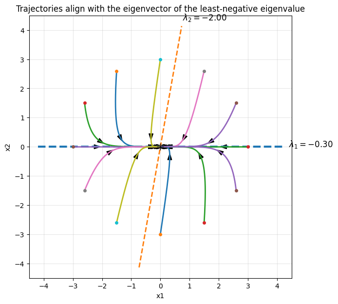
Case 1: Assume that \(A \in \mathbb{R}^{2 \times 2}\) has two distinct real eigenvalues \(\lambda_1\) and \(\lambda_2\) with corresponding eigenvectors \(v_1\) and \(v_2\).

Then,

\[\begin{split} x(t) = e^{A t} x_0 = \begin{bmatrix} v_1 & v_2 \end{bmatrix} \begin{bmatrix} e^{\lambda_1 t} & 0 \\ 0 & e^{\lambda_2 t} \end{bmatrix} \begin{bmatrix} v_1 & v_2 \end{bmatrix}^{-1} x_0. \end{split}\]

The solution is therefore a linear combination of \(e^{\lambda_1 t}\) and \(e^{\lambda_2 t}\).

Suppose the initial condition can be written as

\[\begin{split} x_0 = \begin{bmatrix} v_1 & v_2 \end{bmatrix} \begin{bmatrix} \alpha_1 \\ \alpha_2 \end{bmatrix}, \qquad \text{for some } \alpha_1, \alpha_2 \in \mathbb{R}. \end{split}\]

Then,

\[\begin{split} \begin{aligned} x(t) &= \begin{bmatrix} v_1 & v_2 \end{bmatrix} \begin{bmatrix} e^{\lambda_1 t} & 0 \\ 0 & e^{\lambda_2 t} \end{bmatrix} \begin{bmatrix} v_1 & v_2 \end{bmatrix}^{-1} \begin{bmatrix} v_1 & v_2 \end{bmatrix} \begin{bmatrix} \alpha_1 \\ \alpha_2 \end{bmatrix} \\[6pt] &= \alpha_1 e^{\lambda_1 t} v_1 + \alpha_2 e^{\lambda_2 t} v_2. \end{aligned} \end{split}\]

(See the example below for a geometric interpreations of this last observation.)

Case 2: This is the case with complex eigenvalues. The reasoning in case 1 carries over but working with complex eigenvalues and eigenvectors may not be as intuitive. For a more intuitive representation, we need a few more facts.

Let

\[ \lambda = \sigma + j \omega, \qquad v = v_R + j v_I, \]

where \(v_R, v_I \in \mathbb{R}^2\).

The eigenvalue–eigenvector equation

\[ A v = \lambda v \]

can be written as

\[ A (v_R + j v_I) = (\sigma + j \omega)(v_R + j v_I). \]

Expanding both sides gives

\[ A v_R + j A v_I = (\sigma v_R - \omega v_I) + j(\omega v_R + \sigma v_I). \]

Equating real and imaginary parts yields

\[ A v_R = \sigma v_R - \omega v_I, \]

\[ A v_I = \omega v_R + \sigma v_I. \]

These equations can be rewritten compactly as

\[\begin{split} A \begin{bmatrix} v_R & v_I \end{bmatrix} = \begin{bmatrix} v_R & v_I \end{bmatrix} \begin{bmatrix} \sigma & \omega \\ -\omega & \sigma \end{bmatrix}. \end{split}\]

Define

\[\begin{split}P = \begin{bmatrix} v_R & v_I \end{bmatrix}, \qquad J_c = \begin{bmatrix} \sigma & \omega \\ -\omega & \sigma \end{bmatrix}. \end{split}\]

Then

\[ A P = P J_c, \]

and equivalently,

\[ A = P J_c P^{-1}. \]

Does

\[\begin{split} J_c = \begin{bmatrix} \sigma & \omega \\ -\omega & \sigma \end{bmatrix} \end{split}\]

look familiar?

We can write

\[\begin{split} e^{J_c t} = e^{\sigma t} \begin{bmatrix} \cos(\omega t) & \sin(\omega t) \\ -\sin(\omega t) & \cos(\omega t) \end{bmatrix}. \end{split}\]

Therefore, the solution of

\[ \dot{x}(t) = A x(t) \]

can be expressed as

\[\begin{split} x(t) = e^{\sigma t}\, T \begin{bmatrix} \cos(\omega t) & \sin(\omega t) \\ -\sin(\omega t) & \cos(\omega t) \end{bmatrix} T^{-1} x_0. \end{split}\]

The solution is a linear combination of

\[ e^{\sigma t} \sin(\omega t) \quad \text{and} \quad e^{\sigma t} \cos(\omega t). \]

Some observations about second-order systems

• The free response for a first-order system could include terms of the form of \(e^{a t}\) where \(a\) is a real number. Therefore, it can not include oscilations.

• The free response for a second-order system may or may not include oscillations.

  • If the eigenvalues are real, the response is a combination of two first-order systems; hence, does not have oscilations.

  • If the eigenvalues are complex, the system has oscillations.

The following example focuses on classifying second-order systems with respect to their eigenvalues.

Alternative represenations of second-order systems

We will work with second-order system quite often. It is therefore useful to familiarize ourselves with two related alternative representations.

The first one simplies stability checks. The second-order system

\[ \ddot{y}(t) + \alpha \dot{y}(t) + \beta y(t) = 0. \]

is asymptotically stable if and only if \(\alpha >0\) and \(\beta >0\).

Here is an explanation of why.

The second one gives an interpretation about intuitive quantities that we often encounter in mechanical or electrical systems.

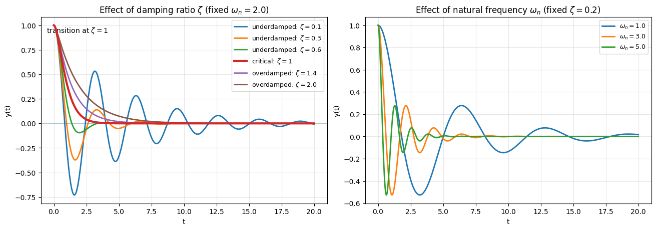
Consider the second-order system

\[ \ddot{y}(t) + 2 \zeta \omega_n \dot{y}(t) + \omega_n^2 y(t) = 0. \]

The roots of the resulting characteristic polynomial are

\[ -\zeta \omega_n \pm j\,\omega_n \sqrt{1 - \zeta^2}. \]

Here,

• \(\zeta\) is the damping ratio, and

• \(\omega_n\) is the natural frequency.

Step response for linear systems

Consider the linear time-invariant (LTI) state-space system

\[ \dot{x}(t) = A x(t) + B u(t), \]

\[ y(t) = C x(t) + D u(t), \]

with initial condition

\[ x(0) = x_0. \]

The matrices have compatible dimensions:

\[ A \in \mathbb{R}^{n \times n}, ~ B \in \mathbb{R}^{n \times m},~ C \in \mathbb{R}^{p \times n}, ~ D \in \mathbb{R}^{p \times m}. \]

Let \(u\) be a step input of the form

\[ u(t) = \bar{u}, \qquad t \ge 0, \]

where

\[ \bar{u} \in \mathbb{R}^m. \]

Recall that, for the scalar case with

\[ A, B, C, D \in \mathbb{R}, \]

the step response was

\[ x(t) = e^{A t} x_0 - \frac{B}{A}\bigl(1 - e^{A t}\bigr)\,\bar{u} \]

and

\[ y(t) = C e^{A t} x_0 - \frac{C B}{A}\bigl(1 - e^{A t}\bigr)\,\bar{u} + D\,\bar{u}. \]

For the general case, the step response looks similar modulo we have to pay attention to matrices. Starting from the general solution of the state equation,

\[ x(t) = e^{A t} x_0 + \int_{0}^{t} e^{A(t-\tau)} B u(\tau)\, d\tau, \]

and considering a step input

\[ u(t) = \bar{u}, \]

we obtain

\[ x(t) = e^{A t} x_0 + \int_{0}^{t} e^{A(t-\tau)} B \bar{u}\, d\tau. \]

Factor out \(e^{A t}\) from the integral:

\[ x(t) = e^{A t} x_0 + e^{A t} \left( \int_{0}^{t} e^{-A \tau}\, d\tau \right) B \bar{u}. \]

Evaluating the matrix integral (assuming \(A\) is invertible, and when the system is stable \(A\) is invertible),

\[ \int_{0}^{t} e^{-A \tau}\, d\tau = \left( -e^{-A \tau} A^{-1} \right)\Big|_{0}^{t}, \]

which gives

\[ \int_{0}^{t} e^{-A \tau}\, d\tau = \left( I - e^{-A t} \right) A^{-1}. \]

Substituting back,

\[ x(t) = e^{A t} x_0 + e^{A t} \left( I - e^{-A t} \right) A^{-1} B \bar{u}. \]

Finally, simplifying,

\[ \boxed{ x(t) = e^{A t} x_0 + \left( e^{A t} - I \right) A^{-1} B \bar{u}. } \]

Using the output equation

\[ y(t) = C x(t) + D u(t), \]

and substituting the expression for \(x(t)\),

\[ x(t) = e^{A t} x_0 + \left( e^{A t} - I \right) A^{-1} B \bar{u}, \]

we obtain

\[ y(t) = C e^{A t} x_0 + C\left( e^{A t} - I \right) A^{-1} B \bar{u} + D \bar{u}. \]

Rearranging terms,

\[ y(t) = C e^{A t} x_0 - C A^{-1} B \bar{u} + C e^{A t} A^{-1} B \bar{u} + D \bar{u}. \]

Grouping the exponential terms,

\[ y(t) = C e^{A t}\left( x_0 + A^{-1} B \bar{u} \right) + \left( D - C A^{-1} B \right)\bar{u}. \]

Equivalently, this can be written as

\[ \boxed{ y(t) = C e^{A t}\left( x_0 - \left(-A^{-1} B \bar{u}\right) \right) + \left( D - C A^{-1} B \right)\bar{u}. } \]

Steady-state response under a step input

Recall

\[ y(t)=C e^{At}\Bigl(x_0-(-A^{-1}B\bar{u})\Bigr)+\bigl(D-CA^{-1}B\bigr)\bar{u}. \]

When does a steady-state value exist?

If

\[ \operatorname{Re}(\lambda_i(A))<0 \quad \text{for all } i=1,\dots,n, \]

then

\[ e^{At}\to 0_{n\times n}\quad \text{as } t\to\infty. \]

Therefore the transient term \(C e^{At}(\cdot)\) vanishes, and the output converges to a constant.

As \(t\to\infty\), \(y(t)\) approaches

\[ \boxed{y_{\mathrm{ss}} =\bigl(D-CA^{-1}B\bigr)\bar{u}.} \]

Note that \(y_{ss}\) does not depent on \(x_0\).

When \(u,y\in\mathbb{R}\) (single-input, single-output), \(\bigl(D-CA^{-1}B\bigr)\) is a scalar, and

\[ y_{\mathrm{ss}}=\bigl(D-CA^{-1}B\bigr)\bar{u}, \]

so the steady-state gain from \(u\) to \(y\) is

\[\boxed{ \frac{y_{\mathrm{ss}}}{\bar{u}}=D-CA^{-1}B.} \]

Example: Steady-state gain for a second-order system (in an “alternate” form)

Consider the second-order system

\[ \ddot{q}(t) + a_1 \dot{q}(t) + a_2 q(t) = b_1 \,\bar{u}, \]

where \(\bar{u}\) is a constant (step) input.

Assume the system is stable, i.e.,

\[ a_1 > 0, \qquad a_2 > 0. \]

Let us obtain a state space representation and apply the result we derived above. Define the state variables

\[ x_1 = q, \qquad x_2 = \dot{q}. \]

Then the system can be written in state-space form as

\[\begin{split} \dot{x} = \begin{bmatrix} 0 & 1 \\ - a_2 & - a_1 \end{bmatrix} x + \begin{bmatrix} 0 \\ b_1 \end{bmatrix} \bar{u}, \end{split}\]

with output

\[ y = \begin{bmatrix} 1 & 0 \end{bmatrix} x. \]

Check whether the outcome here will depend on the choice of the states.

Since the system is stable, the steady-state output exists. Using the steady-state gain formula,

\[ y_{\mathrm{ss}} = - C A^{-1} B \,\bar{u}, \]

we obtain

\[ - C A^{-1} B = \frac{b_1}{a_2}. \]

Thus, the steady-state gain from the input \(\bar{u}\) to the output ( y ) is

\[ \frac{y_{\mathrm{ss}}}{\bar{u}} = \frac{b_1}{a_2}. \]

This provides a simple way to compute the steady-state gain for second-order systems in this alternative form.

Matching exercise: step responses of a second-order system

Consider the second-order system

\[ \ddot{y}(t) + 2\zeta\omega_n \dot{y}(t) + \omega_n^2 y(t) = b\,\omega_n^2\,u(t), \]

with unit-step input \(u(t)=1\) for \(t\ge 0\) and zero initial conditions.

The figure below shows 12 step responses, generated using the parameter sets

\[ \zeta \in \{0.9,\;0.65,\;0.3\}, \qquad \omega_n \in \{1,\;5\}, \qquad b \in \{1,\;3\}. \]

For each subplot (System 1–12), identify the corresponding values of \(\zeta\), \(\omega_n\), and \(b\).

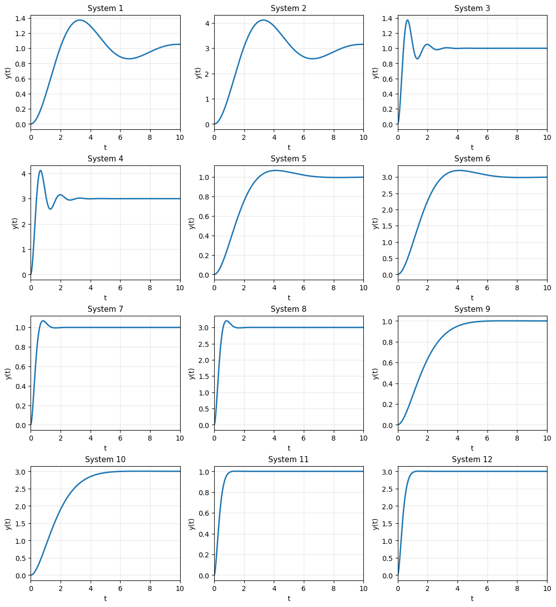
	ζ	ωₙ	b
System
1	0.30	1.0	1.0
2	0.30	1.0	3.0
3	0.30	5.0	1.0
4	0.30	5.0	3.0
5	0.65	1.0	1.0
6	0.65	1.0	3.0
7	0.65	5.0	1.0
8	0.65	5.0	3.0
9	0.90	1.0	1.0
10	0.90	1.0	3.0
11	0.90	5.0	1.0
12	0.90	5.0	3.0