![]()
All rights reserved. For enrolled students only. Redistribution prohibited.
State Estimation#
Motivation for state estimation#
In previous lectures we designed controllers of the form
for the open-loop dynamics
so that the closed-loop dynamics
have desired stability and transient properties.
However, this control law assumes that all components of the state vector \(x(t)\) are available for measurement.
In many practical systems this assumption is not realistic.
Examples include:
Aircraft control: pitch angle may be measured, but angle of attack may not be directly measurable.
Robotics: position sensors are common, but velocities are often not measured directly.
Process control: internal states such as concentrations or temperatures inside reactors are not accessible.
Therefore, if the full state \(x(t)\) is not available, we need a way to construct an estimate
of \(x(t)\) using the available signals:
the control input \(u(t)\), and
the measured output \(y(t)\).
This leads to the problem of state estimation, where we design a dynamical system, called an observer, that reconstructs the state from measurements.
Once an estimate \(\bar{x}(t)\) is available, we can implement the controller
which approximates the ideal state-feedback law.
Constructing a state estimate#
Suppose the system is
We want to construct an estimate \(\bar{x}(t)\) of the state \(x(t)\) using the available signals \(u(t)\) and \(y(t)\).
A natural starting point is to simulate the system dynamics:
However, if the initial condition \(\bar{x}(0)\) is not equal to \(x(0)\), then this model will generally produce the wrong trajectory.
To correct this, we use the measurement \(y(t)\).
The estimated output is
The difference
represents the output estimation error. We can use this error to adjust the estimate.
This leads to the observer dynamics
where \(L\) is the observer gain matrix.
This dynamical system is called a Luenberger observer.
Estimation of error dynamics#
To understand how well the observer performs, define the estimation error
We can derive the dynamics of this error by subtracting the observer equation from the plant equation.
The plant dynamics are
and the observer dynamics are
Subtracting the two equations gives
Substitute the expressions above:
Cancel the terms involving \(Bu(t)\) and rearrange:
Since \(e(t) = x(t) - \bar{x}(t)\), the estimation error evolves according to the linear system
Therefore, if the eigenvalues of \(A - LC\) have negative real parts, then
In that case, the estimate \(\bar{x}(t)\) converges to the true state \(x(t)\).
Observer design#
The matrix \(L\) can be chosen to shape the eigenvalues of \(A - LC\).
This problem is closely related to the state-feedback design problem. Recall that with state feedback
the closed-loop dynamics become
In that case, the gain \(K\) is selected to place the eigenvalues of \(A - BK\) at desired locations.
Similarly, in observer design we select \(L\) so that the eigenvalues of \(A - LC\) lie in desired locations in the complex plane.
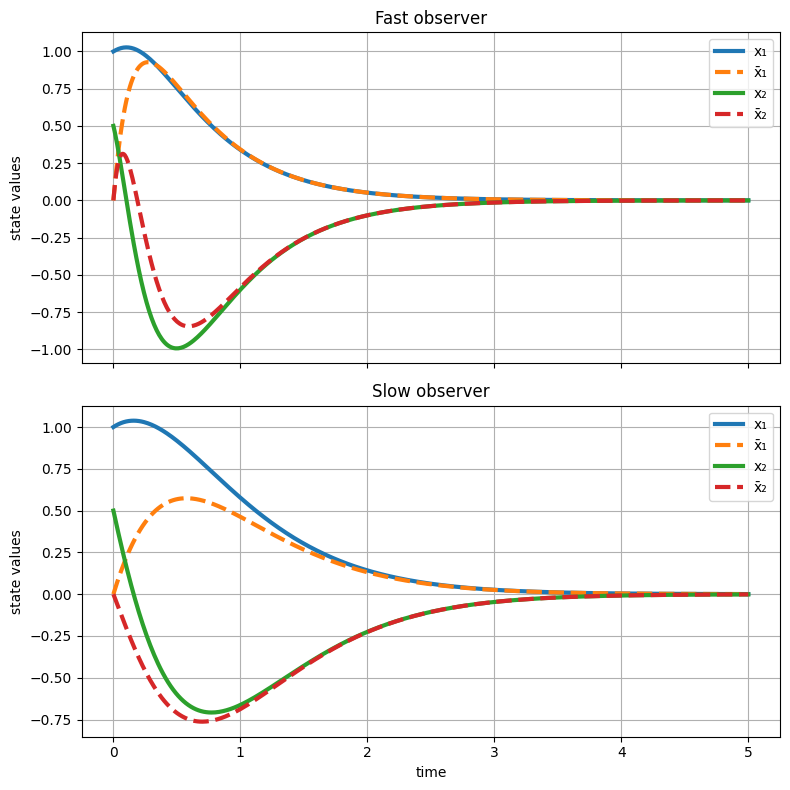
In practice, the eigenvalues of \(A - LC\) are typically chosen to have larger negative real parts than the eigenvalues of \(A - BK\).
A common rule of thumb is to select the eigenvalues of \(A - LC\) so that they correspond to dynamics that are roughly 3–10 times faster than those of \(A - BK\).
This ensures that the estimation error decays quickly relative to the system dynamics, so that \(\bar{x}(t)\) rapidly approaches the true state \(x(t)\).
Observer-based state feedback#
Suppose we have designed a state-feedback controller
so that the eigenvalues of \(A - BK\) give the desired closed-loop behavior.
If the full state \(x(t)\) is not available for measurement, we instead use the state estimate \(\bar{x}(t)\) produced by the observer:
The plant and observer then evolve according to
Substituting the control law \(u(t) = -K \bar{x}(t)\) gives
Recall the estimation error
Using this definition, the closed-loop dynamics can be written as
Separation Principle#
The matrix governing the combined dynamics is upper triangular:
For an upper triangular matrix, the eigenvalues are exactly the union of the eigenvalues of the diagonal blocks. Therefore, the eigenvalues of the combined observer-based closed-loop system are
the eigenvalues of \(A-BK\), and
the eigenvalues of \(A-LC\).
This means that the controller gain \(K\) and the observer gain \(L\) can be designed independently.
This result is known as the separation principle.
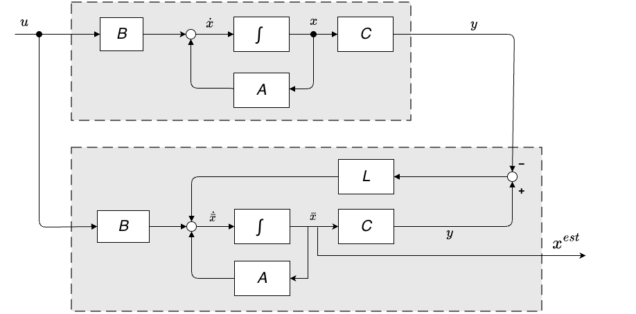
The block diagram below illustrates the interaction between the plant and observer dynamics.
Example: Designing a Controller and Observer#
Consider the system
The goal is to design
a state-feedback controller
\[ u(t) = -Kx(t), \]and an observer
\[ \dot{\bar{x}}(t) = A\bar{x}(t) + Bu(t) + L(y(t) - C\bar{x}(t)), \]
so that the closed-loop system has desired behavior.
Step 1: Design the controller
Choose the gain \(K\) so that the eigenvalues of
are placed at desired locations.
For example, we may choose eigenvalues at
This determines the gain \(K\).
Step 2: Design the observer
Choose the gain \(L\) so that the eigenvalues of
are placed further to the left in the complex plane.
For example,
This ensures that the estimation error
decays faster than the system dynamics.
Step 3: Implement the observer-based controller
The controller now uses the estimated state:
The plant and observer operate together as
Because of the separation principle, the eigenvalues of the combined system consist of
the eigenvalues of \(A-BK\) and
the eigenvalues of \(A-LC\).
Controller gain K: [[4. 2.]]
Fast observer gain L:
 [[10.]
 [10.]]
Slow observer gain L:
 [[ 2.5]
 [-2. ]]