All rights reserved. For enrolled students only. Redistribution prohibited.

Introduction to control design

What will we cover?

• What is design?

• Design specifications

• Design examples

What do we mean by design?

Up to this point, we have focused on analysis: given a model and a controller, we studied how the system behaves. Design reverses this perspective.

In control design, the goal is to choose a controller so that the closed-loop system behaves in a desired way.

In other words, design answers the question: How should we modify the system, through feedback, to achieve behavior we want?

For now, we will focus on relatively simple controllers and relatively simple systems, but the underlying idea applies much more broadly.

Specifications: design for what?

Design is meaningless without a notion of desired behavior. These desired behaviors are expressed through specifications.

Specifications describe what we want the system to do, rather than how it should be implemented.

To make the idea of design specifications concrete, we begin with a simple and widely used example: the step response of a second-order system.

Although real systems may be higher order, many closed-loop responses are well approximated by second-order behavior. As a result, the qualitative features of second-order responses play a central role in control design.

The figure below shows the response of a stable, underdamped second-order system to a unit-step input. This type of response is often considered “typical” and serves as a reference for discussing desired behavior.

Several key properties of the step response can be read directly from the figure:

• Stability
  The closed-loop stability is a prerequisite for discussing all other specifications.

• Steady-state value \(y_{ss}\)
  The value approached by the output as time goes to infinity.

• Overshoot \(M_p\)
  The maximum amount by which the response exceeds its steady-state value, expressed as a percentage of \(y_{ss}\).

• Rise time \(T_r\)
  The time required for the response to rise from a small fraction of its steady-state value to a large fraction (commonly \(10\%\) to \(90\%\)).

• Settling time \(T_s\)
  The time after which the response remains within a specified tolerance band (typically \(2\%\) or \(5\%\)) around the steady-state value.

These quantities provide a convenient way to translate qualitative goals such as “fast,” “smooth,” or “well-damped” into quantitative design specifications.

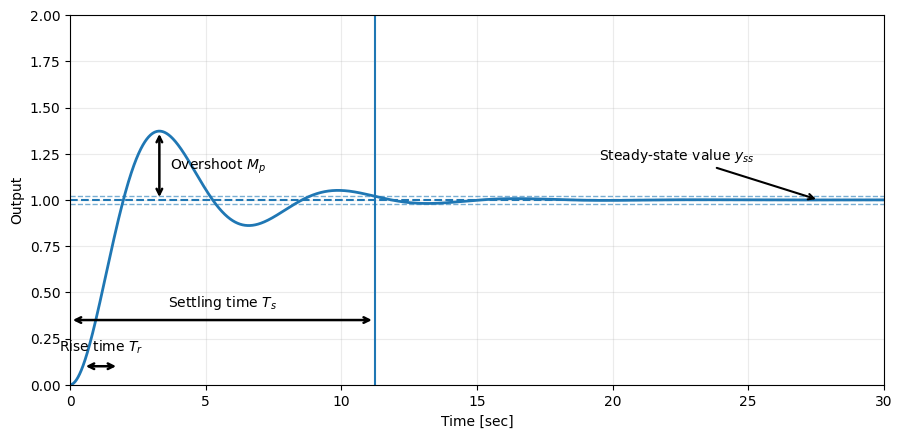
zeta = 0.3, wn = 1.0
y_ss = 1.0
Overshoot Mp = 37.2%
Rise time Tr = 1.32 s (10% to 90%)
Settling time Ts = 11.23 s (2% band)

Different ways to express design specifications

The step response example illustrates one important way of describing desired behavior: time-domain specifications. However, design specifications in control can be expressed in several different forms, depending on what aspects of the system behavior are most important and how the designer intends to carry out the design.

There is no single “correct” way to specify performance. Different representations emphasize different features of the system.

Below are some common ways in which specifications are expressed in control.

Time-domain specifications

Time-domain specifications describe how the system responds over time to inputs, such as steps or disturbances.

Examples include:

• stability (convergence to a steady state),

• rise time,

• overshoot,

• settling time,

• steady-state error.

Steady-state specifications

Steady-state specifications focus on the long-term behavior of the system, independent of transients.

Examples include:

• desired steady-state value,

• zero steady-state error to a step input,

• steady-state gain.

Frequency-domain specifications

Frequency-domain specifications describe how the system responds to sinusoidal inputs of different frequencies.

Examples include:

• bandwidth,

• gain and phase margins,

• attenuation or amplification in certain frequency ranges.

These specifications may be particularly useful for understanding robustness to disturbances and noise.

Pole- or eigenvalue-based specifications

Some specifications are expressed directly in terms of the system’s dynamics.

Examples include:

• locations of closed-loop poles,

• damping ratio and natural frequency,

• bounds on real parts of eigenvalues.

These specifications connect directly to stability and transient behavior and are often used in analytical design methods.

Qualitative or application-driven specifications

In many applications, specifications are stated informally, such as:

• “fast but not oscillatory,”

• “smooth response,”

• “robust to disturbances,”

• “no large actuator effort.”

A key task in control design is to translate such qualitative goals into precise, quantitative specifications.

Different forms of specifications often describe the same (or similar) desired behavior, but in different languages.

The choice of representation depends on:

• what behavior matters in the application,

• what measurements are available,

• and which design tools will be used.

Example: From time-domain specifications to damping ratio (\(\zeta\)) and natural frequency (\(\omega_n\)) to and pole/eigenvalue locations (second-order systems)

A convenient “design language” for many second-order closed-loop responses is the pair \((\zeta,\omega_n)\), where \(\zeta\) is the damping ratio and \(\omega_n\) is the natural frequency.

We start from the canonical second-order model (unit-step input (u(t)=1)):

\[ \ddot y(t) + 2\zeta\omega_n \dot y(t) + \omega_n^2 y(t) = \omega_n^2 u(t). \]

The corresponding characteristic polynomial is

\[ s^2 + 2\zeta\omega_n s + \omega_n^2 = 0, \]

so the (closed-loop) poles are

\[ s_{1,2} = -\zeta\omega_n \;\pm\; j\,\omega_n\sqrt{1-\zeta^2} \quad (0\le \zeta < 1). \]

It is often helpful to define the decay rate \(\sigma\) and the damped frequency \(\omega_d\):

\[ \sigma := \zeta\omega_n, \qquad \omega_d := \omega_n\sqrt{1-\zeta^2}, \]

so that the roots of the characteristic polynomial are

\[ s_{1,2} = -\sigma \pm j\,\omega_d. \]

Time-domain quantities in terms of \(\zeta\) and \(\omega_n\)

For the underdamped case \(0\le \zeta < 1\), several standard step-response measures are approximately related to \(\zeta\) and \(\omega_n\).

Overshoot. The (fractional) peak overshoot (M_p) satisfies

\[ M_p = \exp\!\left(\frac{-\pi\zeta}{\sqrt{1-\zeta^2}}\right), \qquad 0\le \zeta < 1. \]

Peak time. The time of the first peak is

\[ T_p = \frac{\pi}{\omega_d} = \frac{\pi}{\omega_n\sqrt{1-\zeta^2}}. \]

Settling time. Using the envelope \(e^{-\sigma t}\) and a tolerance \(\varepsilon\), a common approximation is

\[ T_s \approx \frac{-\ln(\varepsilon)}{\sigma} = \frac{-\ln(\varepsilon)}{\zeta\omega_n}. \]

For example:

• 2% settling \((\varepsilon=0.02\)) gives \(T_s \approx \frac{4}{\zeta\omega_n}\),

• 1% settling (\(\varepsilon=0.01\)) gives \(T_s \approx \frac{4.6}{\zeta\omega_n}\).

Rise time. There are multiple rise-time conventions (10–90%, 0–100%, etc.), so the formula depends on which definition is used. A commonly used rough rule of thumb for moderate damping is

\[ T_r \approx \frac{1.8}{\omega_n}. \]

Translating specifications \(\rightarrow\) pole/eigenvalue locations

An example workflow:

1. Pick \(\zeta\) from overshoot.
   Overshoot depends primarily on \(\zeta\). For a target \(M_p\), solve

   \[ M_p = \exp\!\left(\frac{-\pi\zeta}{\sqrt{1-\zeta^2}}\right) \]

   for \(\zeta\).

2. Pick \(\omega_n\) from speed.
   Speed measures depend on \(\zeta\omega_n\) (settling) and \(\omega_n\) (rough rise time). For example, using settling time (2%):

   \[ T_s \approx \frac{4}{\zeta\omega_n} \quad\Rightarrow\quad \omega_n \approx \frac{4}{\zeta T_s}. \]

3. Convert to pole locations.
   Once \((\zeta,\omega_n)\) are selected, the desired pole pair is

   \[ s_{1,2} = -\zeta\omega_n \pm j\,\omega_n\sqrt{1-\zeta^2}. \]

Geometrically, \(\zeta\omega_n\) sets how fast transients decay (how far left the poles are), while \(\omega_n\sqrt{1-\zeta^2}\) sets the oscillation frequency (how high the poles are above and below the real axis).

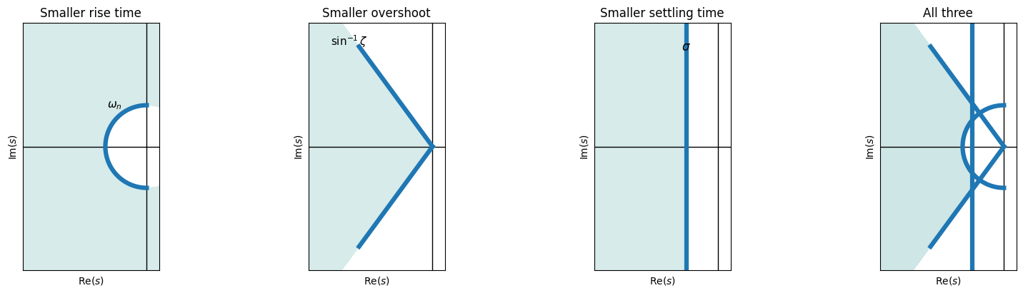
Interpreting time-domain specifications in the complex plane

The figure below illustrates how common time-domain design specifications for second-order systems translate into constraints on closed-loop pole (or eigenvalue) locations in the complex plane.

Rise time: A smaller rise time corresponds to a larger natural frequency \(\omega_n\). Since second-order poles satisfy \(|s|=\omega_n\), the rise-time requirement excludes pole locations close to the origin.

The shaded region indicates pole locations with

\[ \omega_n \ge \omega_{n,\min}, \]

that is, poles lying outside the circle of radius \(\omega_{n,\min}\).

Overshoot: Overshoot is determined primarily by the damping ratio \(\zeta\). For underdamped poles (i.e., \(\zeta<1\)), \(\zeta\) depends on the angle of the pole relative to the negative real axis.

The shaded wedge corresponds to pole locations satisfying

\[ \zeta \ge \zeta_{\min}, \]

which restricts poles to lie closer to the negative real axis and limits oscillatory behavior.

Settling time: Settling time is governed by the exponential decay rate \(\sigma\), which is the magnitude of the real part of the poles.

The shaded region indicates pole locations satisfying

\[ \mathrm{Re}(s) \le -\sigma_{\min}, \]

which pushes poles farther to the left in the complex plane, ensuring faster decay of transients.

Combined specifications: In practice, multiple specifications must be satisfied simultaneously. The rightmost panel shows the intersection of the rise-time, overshoot, and settling-time constraints.

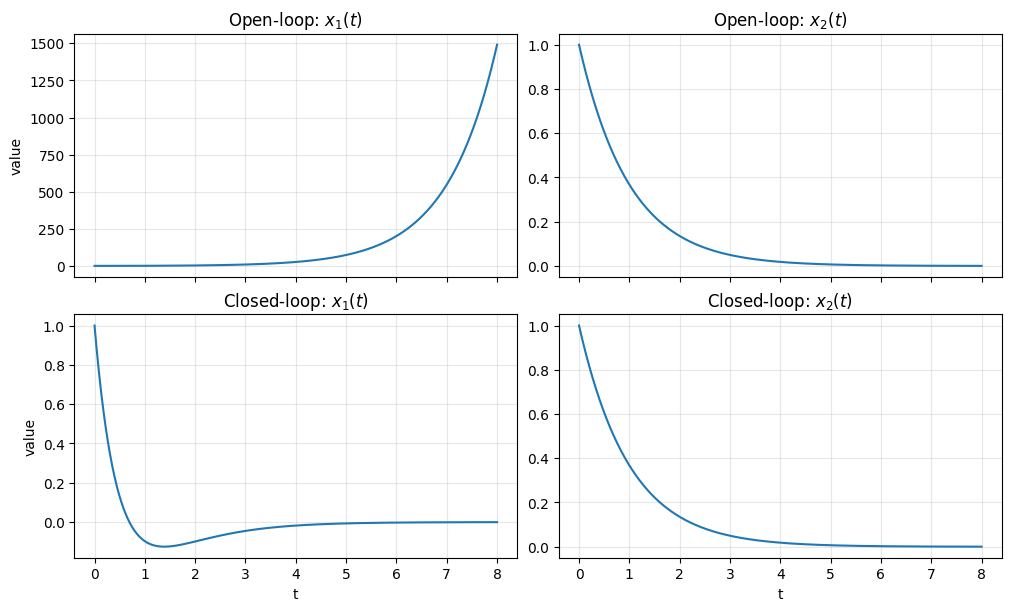
Design Example 1: State-feedback stabilization of a linear system

Consider the linear system

\[\begin{split} \dot{x} = \begin{bmatrix} 1 & -1 \\ 0 & -1 \end{bmatrix} x + \begin{bmatrix} 1 \\ 0 \end{bmatrix} u, \end{split}\]

which we write compactly as

\[ \dot{x} = A x + B u. \]

Is the open-loop system stable?

The eigenvalues of the matrix

\[\begin{split} A = \begin{bmatrix} 1 & -1 \\ 0 & -1 \end{bmatrix} \end{split}\]

are

\[ \lambda_1 = 1, \qquad \lambda_2 = -1. \]

Since one eigenvalue has positive real part, the open-loop system is not stable.

Specification

Design a state-feedback controller

\[ u = Kx, \qquad K \in \mathbb{R}^{1 \times 2}, \]

such that the resulting closed-loop system is stable.

Closed-loop dynamics

Substituting (u = Kx) into the system gives

\[ \dot{x} = A x + B u = A x + B K x = (A + B K)x. \]

Thus, the closed-loop system matrix is

\[\begin{split} A + B K = \begin{bmatrix} 1 & -1 \\ 0 & -1 \end{bmatrix} + \begin{bmatrix} 1 \\ 0 \end{bmatrix} \begin{bmatrix} k_1 & k_2 \end{bmatrix} = \begin{bmatrix} 1 + k_1 & -1 + k_2 \\ 0 & -1 \end{bmatrix}. \end{split}\]

Closed-loop stability condition

The eigenvalues of \(A + BK\) are

\[ \lambda_1 = 1 + k_1, \qquad \lambda_2 = -1. \]

The closed-loop system is stable if and only if

\[ \operatorname{Re}(\lambda_i) < 0 \quad \text{for } i=1,2. \]

Since \(\lambda_2 = -1 < 0\), stability requires

\[ 1 + k_1 < 0. \]

Any controller gain \(K = [k_1\;\;k_2]\) satisfying

\[ k_1 < -1 \]

renders the closed-loop system stable.

The parameter \(k_2\) can be chosen arbitrarily, since it does not affect the closed-loop eigenvalues in this example.

Design Example 2: Integral and proportional–integral control for a first-order system with disturbance

Given

Consider the first-order linear plant with control input \(u\) and disturbance \(d\):

\[ \dot{x}(t) = 2x(t) + u(t) + d(t), \qquad y(t) = x(t). \]

Part 1: Integral control

We first consider an integral (I) controller, defined by

\[ u(t) = K_I z(t), \qquad \dot{z}(t) = r(t) - y(t), \]

where:

• \(z\) is the integral of the tracking error,

• \(r\) is a reference input,

• \(K_I\) is the integral gain.

System block diagram

The following block diagram shows the main components and signal flow for the system.

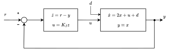
Closed-loop dynamics with integral control

Substituting \(u(t) = K_I z(t)\) and \(y(t)=x(t)\), the closed-loop system becomes

\[\begin{split} \begin{aligned} \dot{x} &= 2x + K_I z + d, \\ \dot{z} &= -x + r. \end{aligned} \end{split}\]

In state-space form,

\[\begin{split} \begin{bmatrix} \dot{x} \\ \dot{z} \end{bmatrix} = \begin{bmatrix} 2 & K_I \\ -1 & 0 \end{bmatrix} \begin{bmatrix} x \\ z \end{bmatrix} + \begin{bmatrix} 1 \\ 0 \end{bmatrix} d + \begin{bmatrix} 0 \\ 1 \end{bmatrix} r. \end{split}\]

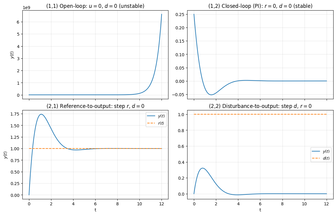
Stability analysis (integral control only)

The characteristic polynomial of the closed-loop A-matrix is

\[ \det(\lambda I - A) = \lambda^2 - 2\lambda + K_I. \]

This polynomial cannot have both roots with negative real parts for any choice of \(K_I\). Therefore, integral (I) control alone cannot stabilize this system.

Part 2: Proportional–integral control

We now consider a proportional–integral (PI) controller, defined by

\[ u(t) = K_I z(t) + K_P\bigl(r(t) - y(t)\bigr), \qquad \dot{z}(t) = r(t) - y(t), \]

where:

• \(K_P\) is the proportional gain,

• \(K_I\) is the integral gain.

Closed-loop dynamics with proportional–integral (PI) control

Substituting \(u\) and \(y\) gives

\[\begin{split} \begin{aligned} \dot{x} &= 2x + K_I z + K_P r - K_P x + d, \\ \dot{z} &= -x + r. \end{aligned} \end{split}\]

In state-space form,

\[\begin{split} \begin{bmatrix} \dot{x} \\ \dot{z} \end{bmatrix} = \begin{bmatrix} 2 - K_P & K_I \\ -1 & 0 \end{bmatrix} \begin{bmatrix} x \\ z \end{bmatrix} + \begin{bmatrix} 1 \\ 0 \end{bmatrix} d + \begin{bmatrix} K_P \\ 1 \end{bmatrix} r. \end{split}\]

Stability conditions (PI control)

The characteristic polynomial of the closed-loop system is

\[ \det(\lambda I - A_{\text{cl}}) = \lambda^2 + (K_P - 2)\lambda + K_I. \]

For stability, the coefficients must satisfy

\[ K_P - 2 > 0, \qquad K_I > 0. \]

Thus, the closed-loop system is stable if and only if

\[ K_P > 2, \qquad K_I > 0. \]

Further questions

Assuming \(K_P\) and \(K_I\) are chosen to satisfy the stability conditions above, determine:

• the closed-loop damping ratio,

• the closed-loop steady-state gain from \(r\) to \(y\),

• the closed-loop steady-state gain from \(d\) to \(y\).

Assume we use a proportional–integral (PI) controller

\[ u(t)=K_I z(t) + K_P\bigl(r(t)-y(t)\bigr), \qquad \dot z(t)=r(t)-y(t), \]

with \(y=x\).

For the closed-loop dynamics, substituting the controller into the plant equations gives

\[\begin{split} \begin{aligned} \dot x &= 2x + K_I z + K_P r - K_P x + d,\\ \dot z &= -x + r. \end{aligned} \end{split}\]

This can be written in state-space form as

\[\begin{split} \begin{bmatrix}\dot x\\ \dot z\end{bmatrix} = \begin{bmatrix} 2-K_P & K_I\\ -1 & 0 \end{bmatrix} \begin{bmatrix}x\\ z\end{bmatrix} + \begin{bmatrix}K_P\\ 1\end{bmatrix} r + \begin{bmatrix}1\\ 0\end{bmatrix} d, \end{split}\]

with output

\[\begin{split} y= \begin{bmatrix}1 & 0\end{bmatrix} \begin{bmatrix}x\\ z\end{bmatrix}. \end{split}\]

For later reference, we define

\[\begin{split} A_{\mathrm{cl}}= \begin{bmatrix} 2-K_P & K_I\\ -1 & 0 \end{bmatrix}, \qquad B_r= \begin{bmatrix}K_P\\ 1\end{bmatrix}, \qquad B_d= \begin{bmatrix}1\\ 0\end{bmatrix}, \qquad C= \begin{bmatrix}1 & 0\end{bmatrix}. \end{split}\]

The characteristic polynomial of the closed-loop system matrix \(A_{\mathrm{cl}}\) is

\[ \det(\lambda I-A_{\mathrm{cl}}) = \lambda^2+(K_P-2)\lambda+K_I. \]

For the closed-loop damping ratio, match \(\lambda^2+(K_P-2)\lambda+K_I\) to the standard second-order form

\[ \lambda^2+2\zeta\omega_n\,\lambda+\omega_n^2. \]

This gives

\[ \omega_n^2=K_I,\qquad 2\zeta\omega_n=K_P-2. \]

So

\[ \omega_n=\sqrt{K_I},\qquad \zeta=\frac{K_P-2}{2\sqrt{K_I}}. \]

Move to the closed-loop steady-state gain from \(r\) to \(y\) now.

\[\begin{split} \text{Gain}_{r \to y} = - \begin{bmatrix} 1 & 0 \end{bmatrix} \begin{bmatrix} 2 - K_P & K_I \\ -1 & 0 \end{bmatrix}^{-1} \begin{bmatrix} K_P \\ 1 \end{bmatrix} \end{split}\]

\[\begin{split} = - \begin{bmatrix} 1 & 0 \end{bmatrix} \frac{1}{K_I} \begin{bmatrix} 0 & -K_I \\ 1 & 2 - K_P \end{bmatrix} \begin{bmatrix} K_P \\ 1 \end{bmatrix} \end{split}\]

\[\begin{split} = - \begin{bmatrix} 1 & 0 \end{bmatrix} \frac{1}{K_I} \begin{bmatrix} - K_I \\ 2 \end{bmatrix} = 1. \end{split}\]

Next up: Closed-loop steady-state gain from \(d\) to \(y\).

\[\begin{split} \text{Gain}_{d \to y} = - \begin{bmatrix} 1 & 0 \end{bmatrix} \begin{bmatrix} 2 - K_P & K_I \\ -1 & 0 \end{bmatrix}^{-1} \begin{bmatrix} 1 \\ 0 \end{bmatrix} \end{split}\]

\[\begin{split} = - \begin{bmatrix} 1 & 0 \end{bmatrix} \frac{1}{K_I} \begin{bmatrix} 0 & -K_I \\ 1 & 2 - K_P \end{bmatrix} \begin{bmatrix} 1 \\ 0 \end{bmatrix} = 0. \end{split}\]

These quantities illustrate how proportional–integral (PI) control addresses stability, reference tracking, and disturbance rejection. We will later re-visit such controllers in more depth.

Design Example 3: Proportional–derivative state feedback with disturbance

Given

Consider the second-order plant

\[ \dot{x}_1(t) = x_2(t), \qquad \dot{x}_2(t) = x_1(t) + 2x_2(t) + u(t) + d(t), \]

with output

\[ y(t) = x_1(t). \]

Here, \(u\) is the control input and \(d\) is a disturbance input. Assume that both \(y\) and \(\dot{y}\) are available for feedback.

System block diagram

The following block diagram shows the main components and signal flow for the system.

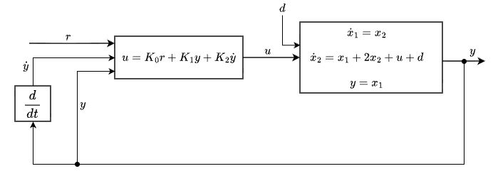
Controller structure

We consider a constant-gain controller with derivative feedback of the form

\[ u(t) = K_0\, r(t) + K_1\, y(t) + K_2\, \dot{y}(t) = K_0\, r(t) + K_1\, x_1(t) + K_2\, x_2(t), \]

where \(r\) is a reference input and \(K_0, K_1, K_2\) are design parameters.

Closed-loop dynamics

Substituting the controller into the plant equations gives

\[\begin{split} \begin{aligned} \dot{x}_1 &= x_2, \\ \dot{x}_2 &= x_1 + 2x_2 + K_1 x_1 + K_2 x_2 + K_0 r + d \\ &= (1+K_1)x_1 + (2+K_2)x_2 + K_0 r + d. \end{aligned} \end{split}\]

In state-space form,

\[\begin{split} \begin{bmatrix} \dot{x}_1 \\ \dot{x}_2 \end{bmatrix} = \begin{bmatrix} 0 & 1 \\ 1+K_1 & 2+K_2 \end{bmatrix} \begin{bmatrix} x_1 \\ x_2 \end{bmatrix} + \begin{bmatrix} 0 \\ K_0 \end{bmatrix} r + \begin{bmatrix} 0 \\ 1 \end{bmatrix} d, \qquad y = \begin{bmatrix}1 & 0\end{bmatrix} \begin{bmatrix}x_1\\x_2\end{bmatrix}. \end{split}\]

Define the closed-loop system matrix

\[\begin{split} A_{\mathrm{cl}} = \begin{bmatrix} 0 & 1 \\ 1+K_1 & 2+K_2 \end{bmatrix}. \end{split}\]

Closed-loop stability and pole placement

The characteristic polynomial of \(A_{\mathrm{cl}}\) is

\[ \det(\lambda I - A_{\mathrm{cl}}) = \lambda^2 + (-2-K_2)\lambda + (-1-K_1). \]

Matching this with the canonical second-order form

\[ \lambda^2 + 2\zeta\omega_n \lambda + \omega_n^2, \]

gives

\[ 2\zeta\omega_n = -2 - K_2, \qquad \omega_n^2 = -1 - K_1. \]

Equivalently,

\[ K_1 = -1 - \omega_n^2, \qquad K_2 = -2 - 2\zeta\omega_n. \]

Thus, by choosing \(\omega_n > 0\) and \(\zeta > 0\), the gains \(K_1\) and \(K_2\) can be selected to place the closed-loop poles at

\[ \lambda_{1,2} = -\zeta\omega_n \pm j\,\omega_n\sqrt{1-\zeta^2}. \]

Steady-state gain from disturbance to output

For a constant disturbance \(d\) and \(r=0\), the steady-state output satisfies

\[ y_{\mathrm{ss}} = -C A_{\mathrm{cl}}^{-1} B_d\, d, \]

where \(B_d = \begin{bmatrix}0 & 1\end{bmatrix}^\top\) and \(C = \begin{bmatrix}1 & 0\end{bmatrix}\).

A direct computation yields

\[ \frac{y_{\mathrm{ss}}}{d} = -\frac{1}{1+K_1}. \]

If \(\omega_n = 1\), then \(K_1 = -2\), and the disturbance-to-output gain becomes

\[ \frac{y_{\mathrm{ss}}}{d} = 1. \]

This shows that one cannot simultaneously fix \(\omega_n\), \(\zeta\), and independently specify the disturbance rejection level using only \(K_1\) and \(K_2\).

Steady-state gain from reference to output

For a constant reference input \(r\) and \(d=0\),

\[ y_{\mathrm{ss}} = -C A_{\mathrm{cl}}^{-1} B_r\, r, \]

where \(B_r = \begin{bmatrix}0 & K_0\end{bmatrix}^\top\).

A direct computation gives

\[ \frac{y_{\mathrm{ss}}}{r} = -\frac{K_0}{1+K_1}. \]

Once \(K_1\) and \(K_2\) are chosen to meet stability and transient specifications, \(K_0\) can be selected independently to achieve the desired steady-state tracking gain.

Key takeaways

• The gains \(K_1\) and \(K_2\) determine the closed-loop poles and therefore stability and transient behavior.

• The gain \(K_0\) does not affect the pole locations and can be used to tune the steady-state reference tracking.

• With a fixed controller structure, it is generally not possible to satisfy an arbitrary number of independent specifications simultaneously.

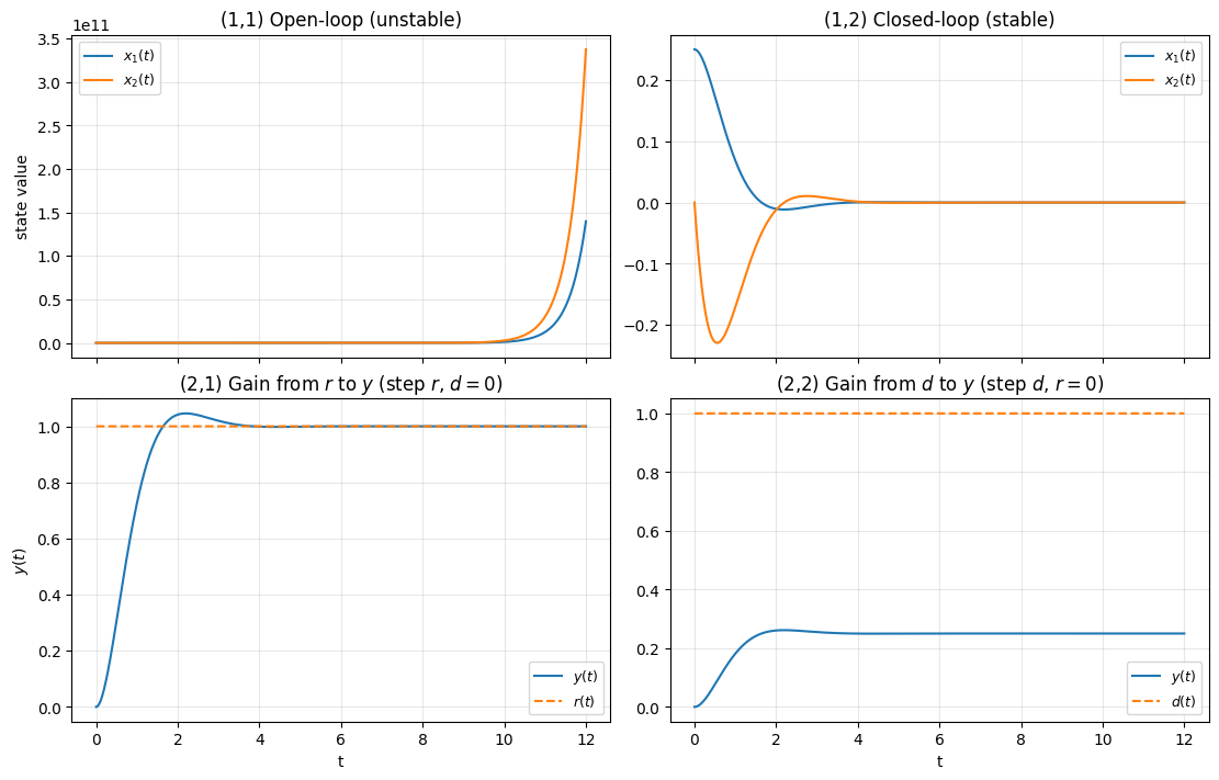
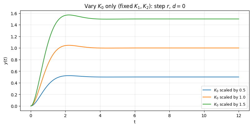
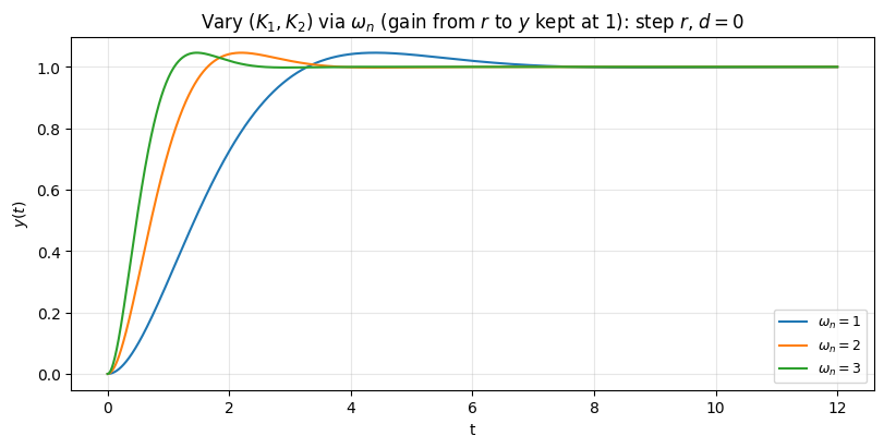
Steady-state gains implied by the chosen parameters:
  zeta=0.70, wn=1.00  ->  gain r->y = 1.000,   gain d->y = 1.000
  zeta=0.70, wn=2.00  ->  gain r->y = 1.000,   gain d->y = 0.250
  zeta=0.70, wn=3.00  ->  gain r->y = 1.000,   gain d->y = 0.111

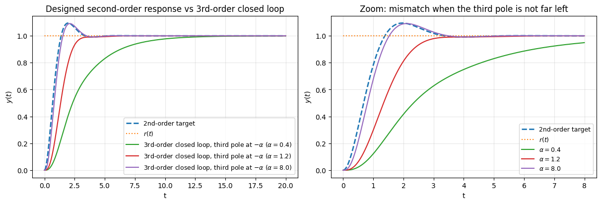
Design Example 4: Making a third-order closed loop behave like a second-order system

Motivation

In the previous examples, the closed-loop dynamics were second order, so we could connect time-domain specifications, such as overshoot and settling time, directly to the damping ratio \(\zeta\) and natural frequency \(\omega_n\) of a canonical second-order model.

In many practical problems, however, the closed-loop system has more than two states. In that case, the second-order formulas do not apply directly, because the transient response is influenced by additional modes.

This example illustrates a common design idea: Design the controller so that the closed-loop has one additional eigenvalue that is much faster than the rest, so the dominant behavior is well-approximated by a second-order model.

Given

Consider a second-order plant with an added integral state (for tracking), so the closed-loop has three states:

\[ \dot{x}(t) = A x(t) + B u(t), \qquad y(t) = C x(t), \]

and define the integral state

\[ \dot{z}(t) = r(t) - y(t). \]

We use an integral-augmented control law of the form

\[ u(t) = -K x(t) + K_I z(t), \]

where \(K \in \mathbb{R}^{1\times 2}\) and \(K_I \in \mathbb{R}\) are design parameters.

The augmented closed-loop state is

\[\begin{split} x_{\mathrm{aug}}(t) = \begin{bmatrix} x(t) \\ z(t) \end{bmatrix} \in \mathbb{R}^3. \end{split}\]

System block diagram

The following block diagram shows the main components and signal flow for the system.

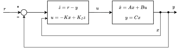
Closed-loop model

The augmented dynamics can be written as

\[\begin{split} \frac{d}{dt}\begin{bmatrix} x \\ z \end{bmatrix} = \begin{bmatrix} A - BK & BK_I \\ -C & 0 \end{bmatrix} \begin{bmatrix} x \\ z \end{bmatrix} + \begin{bmatrix} 0 \\ 1 \end{bmatrix} r. \end{split}\]

Denote the closed-loop matrix by

\[\begin{split} A_{\mathrm{cl}} = \begin{bmatrix} A - BK & BK_I \\ -C & 0 \end{bmatrix}. \end{split}\]

Since \(A_{\mathrm{cl}}\) is \(3\times 3\), it has three eigenvalues:

\[ \lambda_1,\ \lambda_2,\ \lambda_3. \]

Specifications

We would like the overall response to behave approximately like a second-order system with damping ratio \(\zeta\) and natural frequency \(\omega_n\), meaning we want two dominant eigenvalues near

\[ \lambda_{1,2} \approx -\zeta\omega_n \pm j\,\omega_n\sqrt{1-\zeta^2}. \]

However, there is a third eigenvalue \(\lambda_3\). If this third mode is not sufficiently fast, it can noticeably affect the transient response.

To make the third mode negligible in the time window of interest, we impose an additional design requirement:

\[ \lambda_3 \le -\alpha, \]

where \(\alpha\) is chosen large relative to the real part of the dominant pair. A common rule of thumb is

\[ \alpha \ge 5\,\zeta\omega_n \qquad \text{(third mode at least 5 times faster).} \]

Design steps

1. Pick second-order specifications.
   Choose desired overshoot and settling time, translate them into target \((\zeta,\omega_n)\), and compute the desired dominant pole pair

   \[ \lambda_{1,2} = -\zeta\omega_n \pm j\,\omega_n\sqrt{1-\zeta^2}. \]

2. Choose a fast third pole.
   Pick

   \[ \lambda_3 = -\alpha, \]

   with \(\alpha\) much larger than \(\zeta\omega_n\), so this mode decays quickly.

3. Place the closed-loop eigenvalues.

   Select \(K\) and \(K_I\) so that the eigenvalues of \(A_{\mathrm{cl}}\) are

   \[ \{\lambda_1, \lambda_2, \lambda_3\}. \]

4. Interpretation.
   If the third eigenvalue is sufficiently far left, then after a brief initial transient, the output is dominated by the complex pair and looks like a second-order step response with the desired \(\zeta\) and \(\omega_n\).