All rights reserved. For enrolled students only. Redistribution prohibited.

Introduction

What is feedback control about?

Consider balancing a stick on your hand—a simple yet revealing example of feedback control in action.

The system is the stick itself, an inherently “unstable” object that wants to fall. Your hand position is the input you control, and the stick’s angle from vertical is the output you care about.

Sensing happens through your eyes and proprioception. You continuously observe where the stick is leaning and how fast it’s tilting away from vertical.

Based on what you sense, you make control decisions—if the stick leans left, you quickly move your hand left to get underneath it. If it tilts right, you move right. The further and faster it leans, the more aggressively you respond.

Crucially, you close the loop: your hand movement affects the stick’s angle, you sense the new angle, adjust your hand again, and the cycle repeats continuously. This constant feedback loop is what allows you to keep an unstable stick balanced, automatically correcting for disturbances like air currents or initial imperfections in the stick’s position.

Without closing this loop—say, if you moved your hand with your eyes closed—the stick would quickly fall. The power of feedback control lies in this continuous sense-decide-act cycle that enables us to control even unstable systems in uncertain environments.

Open-loop vs. closed-loop control

There are two fundamental types of control systems, distinguished by whether or not they use feedback: open-loop and closed-loop control.

Open-loop control

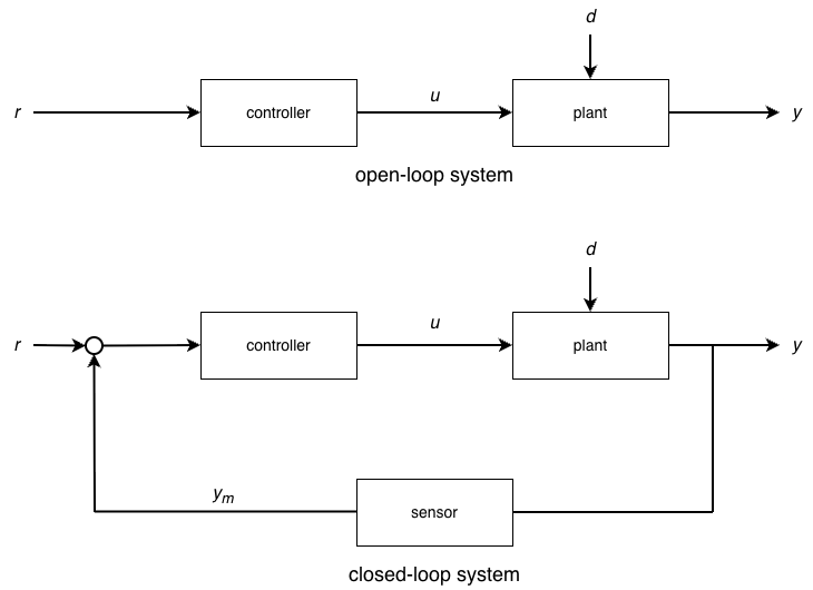
In open-loop control, the controller generates control actions u based solely on the desired reference r, without any measurement of the actual output y. The system operates “blind”—once the control signal is sent to the plant, there is no information about whether the desired result was achieved.

This approach can work for simple, predictable tasks in stable environments. However, it has critical limitations: it cannot compensate for disturbances d that affect the system, it cannot account for uncertainties or changes in the plant’s behavior, and it provides no guarantee that the output matches the reference.

Closed-loop (feedback) control

In closed-loop control, a sensor measures the actual output y (producing measurement y_m) and feeds this information back. This measurement is compared with the desired reference r to compute an error signal. The controller uses this error to determine the control action u.

This feedback path—the loop from output back to input—fundamentally changes what the system can achieve. Closed-loop control automatically corrects for disturbances, adapts to uncertainties in the plant, and continuously adjusts to drive the output toward the reference. The power of feedback lies in this continuous sense-compare-act cycle.

This class is about feedback control!

An illustrative example: aircraft pitch control

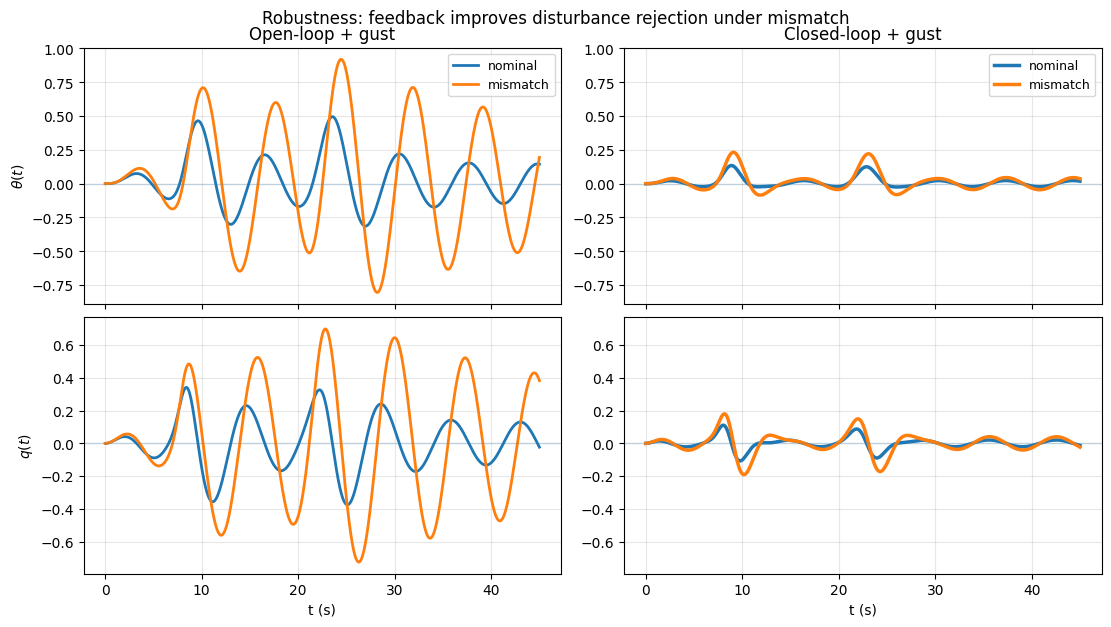
To introduce the central ideas of stability, performance, and robustness in feedback control, we consider a simple model of an aircraft’s pitch motion.

The figure below is a conceptual cartoon of the pitch dynamics, not a full aerodynamic model. It captures three key ingredients: a dynamical system (the aircraft), an actuator (the elevator that controls pitch), and uncertainty or disturbances (such as wind gusts).

Real aircraft dynamics are far more complex, involving intricate aerodynamic effects, structural flexibility, and coupled motions. Yet this simplified model is sufficient to illustrate fundamental control principles. In fact, working with simplified models is standard practice in control engineering—we intentionally use tractable models for analysis and design. Feedback itself helps account for the inevitable errors that arise from model mismatch, as we will discuss later.

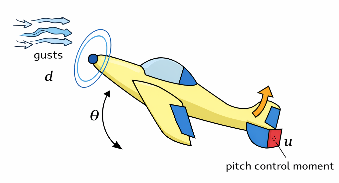
• The aircraft’s pitch angle \(\theta\) describes its orientation.

• The controller applies a pitch control moment \(u\) through the elevator.

• External effects such as wind gusts introduce an unknown disturbance moment \(d\).

• Sensors measure the aircraft motion and provide feedback to the controller.

We describe the aircraft’s pitch motion using a simple linearized model. Define the state variables

\[ \theta = \text{pitch angle}, \qquad q = \dot{\theta} = \text{pitch rate}. \]

The dynamics are modeled as

\[\begin{split} \begin{aligned} \dot{\theta}(t) &= q(t), \\ \dot{q}(t) &= a\,q(t) + b\,\theta(t) + c\,u(t) + d(t), \end{aligned} \end{split}\]

where:

• \(a\) represents aerodynamic damping,

• \(b\) represents pitch stiffness (which may be destabilizing),

• \(c\) represents control effectiveness,

• \(u\) is the pitch control moment commanded by the controller,

• \(d\) is an external disturbance moment due to gusts.

In the “state space” form,

\[\begin{split} x = \begin{bmatrix} \theta \\ q \end{bmatrix}, \qquad \dot{x} = \begin{bmatrix} 0 & 1 \\ b & a \end{bmatrix} x + \begin{bmatrix} 0 \\ c \end{bmatrix} u + \begin{bmatrix} 0 \\ 1 \end{bmatrix} d. \end{split}\]

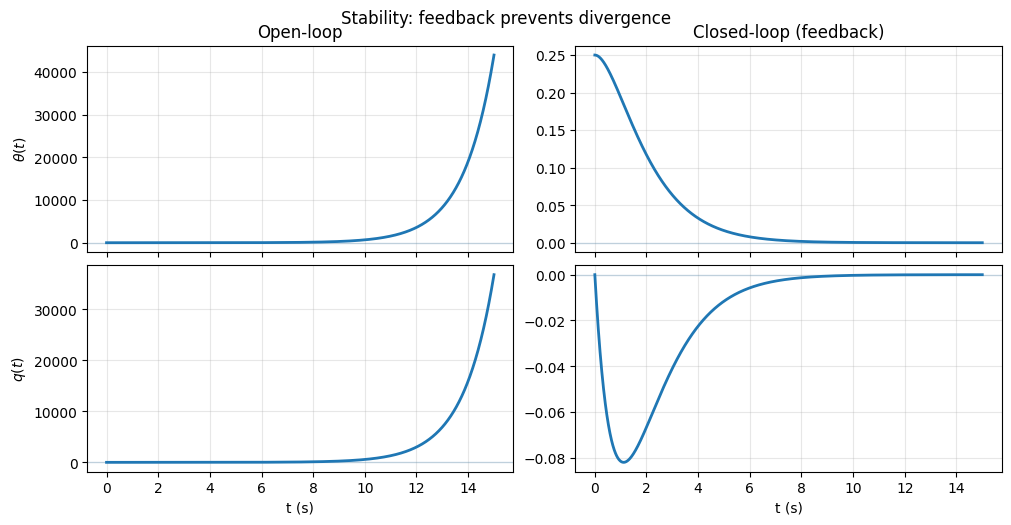
• Stability
  If the aircraft is perturbed—for example, by a wind gust—does it naturally return to its nominal attitude, or does the pitch angle grow without bound? Many systems are inherently unstable or marginally stable. Feedback can stabilize dynamics that would otherwise drift or diverge.

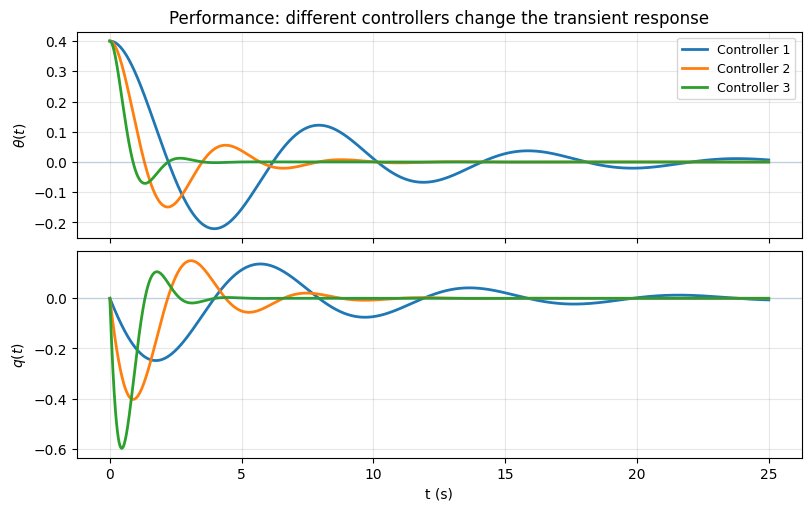
• Performance
  Even when the aircraft is stable, how well does it respond? Does it return to level flight slowly or quickly? Does it overshoot the desired angle or oscillate before settling? Performance concerns the quality of the transient behavior, and different feedback designs can shape the response in dramatically different ways.

• Robustness
  The controller is designed using an approximate model of the aircraft. In reality, parameters such as aerodynamic damping, control effectiveness, and the strength of disturbances are uncertain and may vary with flight conditions. A robust feedback controller continues to perform acceptably even when the actual system differs from the model and when disturbances are present. This is one of feedback control’s most powerful features—the ability to handle uncertainty.

Feedback is everywhere

Feedback control is a unifying idea that appears across engineering, science, technology, and society. Whenever a system must behave reliably in the presence of uncertainty, disturbances, or changing conditions, feedback plays a central role.

Below are representative examples across many domains.

Everyday and classical engineering systems

• Thermostats
  Measure temperature and adjust heating or cooling to maintain a setpoint.

• Cruise control in cars
  Measure vehicle speed and adjust engine power to reject hills and wind.

• Audio systems
  Microphone–speaker feedback can stabilize amplification or cause oscillations (feedback squeal) if poorly designed.

• Manufacturing and industrial automation
  Use feedback to achieve precision, regulate quality, and adapt to variability in materials and operating conditions.

Vehicles, robotics, and autonomous systems

• Aircraft and spacecraft
  Use feedback to stabilize inherently unstable dynamics and reject disturbances such as wind gusts or environmental uncertainty.

• Drones and aerial robots
  Are open-loop unstable and rely entirely on high-rate feedback to fly.

• Robotics
  Use sensor feedback to maintain balance, track trajectories, and interact safely with uncertain environments.

• Autonomous vehicles
  Use feedback to regulate speed, steering, and spacing under changing road and traffic conditions.

Computing, communication, and information systems

• Computer networks and the internet
  Use feedback to manage congestion, allocate bandwidth, and maintain stability.

• Cloud computing and data centers
  Adjust resources in real time based on performance measurements such as latency and load.

• Smartphone cameras and consumer electronics
  Continuously adjust focus, exposure, and stabilization using sensor feedback.

Learning, intelligence, and decision-making systems

• Machine learning and AI
  Use error or reward feedback to update models and improve performance over time.

• Reinforcement learning
  Is explicitly built around feedback from the environment.

• Human learning and education
  Rely on feedback from outcomes, grades, and corrections to guide improvement.

Biological, medical, and ecological systems

• Human balance and motor control
  Use sensory feedback to stabilize posture and coordinate motion.

• Physiological regulation
  Body temperature, glucose levels, and hormone regulation are controlled via feedback loops.

• Medical devices
  Insulin pumps, pacemakers, and anesthesia systems use feedback to ensure safety.

• Ecosystems and population dynamics
  Predator–prey relationships and resource availability form natural feedback loops.

Social, economic, and large-scale systems

• Power grids and energy systems
  Use feedback to regulate frequency, voltage, and balance supply and demand.

• Supply chains and logistics
  Adjust production and inventory based on demand feedback; delays can cause instability (the bullwhip effect).

• Financial markets and automated trading
  Prices respond to actions, and actions respond to prices, forming tight feedback loops.

• Economic and policy systems
  Central banks adjust interest rates based on measured economic indicators.

Fluid, thermal, and propulsion systems

• Aerodynamic flow control
  Measure pressure or velocity and adjust actuators to suppress flow separation and reduce unsteady aerodynamic loads.

• Jet and rocket engines
  Measure chamber pressure or thrust and adjust fuel flow to regulate performance and prevent combustion instabilities.

• Thermal management systems
  Measure temperature and adjust cooling or heating to protect engines, avionics, and thermal protection systems.

• Propellant and fuel systems
  Measure pressure and flow rate and adjust valves to maintain safe and reliable operation under changing conditions.

Less obvious (maybe?) feedback systems

• Noise-canceling headphones
  Measure ambient sound and generate an equal-and-opposite signal to cancel noise in real time.

• Anti-lock braking systems (ABS)
  Measure wheel slip and rapidly modulate braking force to prevent loss of traction.

• Image stabilization (cameras and phones)
  Measure hand motion and adjust sensors or optics to reduce blur during exposure.

• Space telescopes and precision optics
  Measure tiny structural deformations and adjust actuators to maintain alignment at extremely small scales.

• Internet congestion control (e.g., TCP)
  Measure packet loss and delay and adjust transmission rates to avoid network collapse.

• Recommendation and social-media systems
  Measure user engagement and adapt content delivery, forming feedback loops between users and algorithms.

• Anesthesia delivery systems
  Measure patient response and adjust drug dosage to maintain safe levels of sedation.

Representations of dynamical system models

A key idea in feedback control is that the same dynamical system can be represented in multiple, mathematically equivalent forms. Each representation emphasizes different aspects of the system and is useful for answering different questions.

In this course, we will primarily use four representations:

1. Ordinary differential equations (ODEs)

2. State-space models

3. Transfer functions

4. Block diagrams

We use a DC motor as a running example to illustrate how dynamical system models are constructed and how different representations, e.g., ordinary differential equations, state-space models, transfer functions, and block diagrams, arise naturally from the same physical system. (Disclaimer: Understanding how a DC motor is not essential for this part.)

A DC motor couples electrical dynamics and mechanical dynamics. An electrical input produces a mechanical motion, and that motion in turn affects the electrical behavior of the system.

Specifically, the motor consists of:

• a mechanical subsystem, describing the rotation of the motor shaft, and

• an electrical subsystem, describing the armature circuit.

The control input is the armature voltage \(v_a\), which drives an armature current \(i_a\). This current generates a torque that causes the shaft to rotate, producing a shaft angle \(\theta_m\) and angular velocity \(\dot{\theta}_m\). At the same time, the shaft motion induces a back electromotive force (back-emf) that feeds back into the electrical circuit.

This bidirectional coupling makes the DC motor an ideal example for studying feedback control: it is simple enough to analyze explicitly, yet rich enough to demonstrate key concepts such as system order, state variables, and feedback interactions.

(1) ODE representation

Starting from Newton’s law and the armature circuit, we can write the DC motor model directly as coupled ordinary differential equations. In the form shown in the notes:

Mechanical dynamics (second order):

\[ J_m \ddot{\theta}_m + b\,\dot{\theta}_m = k_t i_a. \]

Electrical dynamics (first order):

\[ L_a \frac{d i_a}{dt} + R_a i_a = v_a - k_e \dot{\theta}_m. \]

This representation is closest to the underlying physics and is often how models are first written down.

(2) State-space representation

To obtain a state-space model, we choose state variables

\[\begin{split} x = \begin{bmatrix} \theta_m\\ \dot{\theta}_m\\ i_a \end{bmatrix}, \qquad u = v_a. \end{split}\]

The state-space model has the standard form

\[ \dot{x} = A x + B u, \qquad y = Cx + Du, \]

and for this example (as in the notes),

\[\begin{split} \dot{x} = \begin{bmatrix} 0 & 1 & 0 \\ 0 & -\frac{b}{J_m} & \frac{k_t}{J_m} \\ 0 & -\frac{k_e}{L_a} & -\frac{R_a}{L_a} \end{bmatrix}x + \begin{bmatrix} 0\\ 0\\ \frac{1}{L_a} \end{bmatrix}v_a. \end{split}\]

Depending on what we choose to measure, the output equation may be, for example:

• position output: \(y = \theta_m\),

• speed output: \(y = \dot{\theta}_m\),

• current output: \(y = i_a\), or any combination of these.

(3) Transfer function representation

If we focus on input–output behavior (and assume zero initial conditions), we can represent the motor using a transfer function.

For example, the transfer function from armature voltage to motor angle is

\[ G(s) \;=\; \frac{\Theta_m(s)}{V_a(s)} \;=\; \frac{k_t} {L_a J_m s^3 + (L_a b + R_a J_m)s^2 + (R_a b + k_t k_e)s}. \]

Equivalently, the transfer function from armature voltage to motor speed \(\Omega_m(s)=s\Theta_m(s)\) is

\[ \frac{\Omega_m(s)}{V_a(s)} = \frac{k_t} {(L_a s + R_a)(J_m s + b) + k_t k_e}. \]

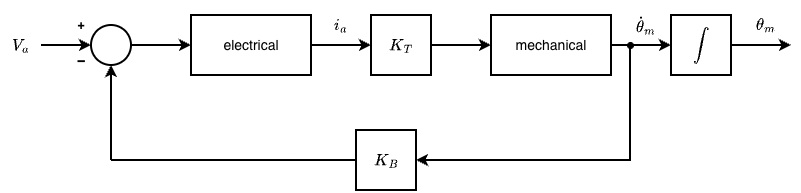
(4) Block diagram representation

A block diagram provides a graphical representation of the model, showing how signals flow between subsystems and how feedback interconnections are formed.

For the DC motor, a natural block diagram view separates:

• the electrical subsystem (voltage \(\to\) current),

• the mechanical subsystem (current \(\to\) torque \(\to\) speed/position),

• the feedback effect of back-emf (speed feeding back into the circuit equation).