All rights reserved. For enrolled students only. Redistribution prohibited.

First-order systems

What are we going to cover?

• Introduce first-order (single-variable) linear ordinary differential equations (ODEs)

• General solution

• Free response and time constants

• Forced response under step and sinusoidal inputs

First-order systems

A first-order (single-variable, i.e., scalar) linear ordinary differential equation (ODE) is represented as

\[ \dot{x}(t) = \frac{dx(t)}{dt} = A x(t) + B u(t), \]

where \(A \in \mathbb{R}\) and \(B \in \mathbb{R}\). Here, \(x(t)\) is the state of the system at time \(t\) and \(u(t)\) is an input to the system at time \(t\). Let \(x_{0} \in \mathbb{R}\) be the initial condition.

You may ask: What makes a differential equation an ordinary differential equation?

What makes an ODE a linear one? Why linear?.

While it does not make much of a difference for first-order systems, the linear system models typically also include an output equation:

\[y(t) = C x(t) + D u(t).\]

Why do we care about first-order systems?

They are the simplest family of models we will encounter, and we will use them to get a sense of several key concepts we will cover throughout the semester.

Example: Cruise control as a first-order system

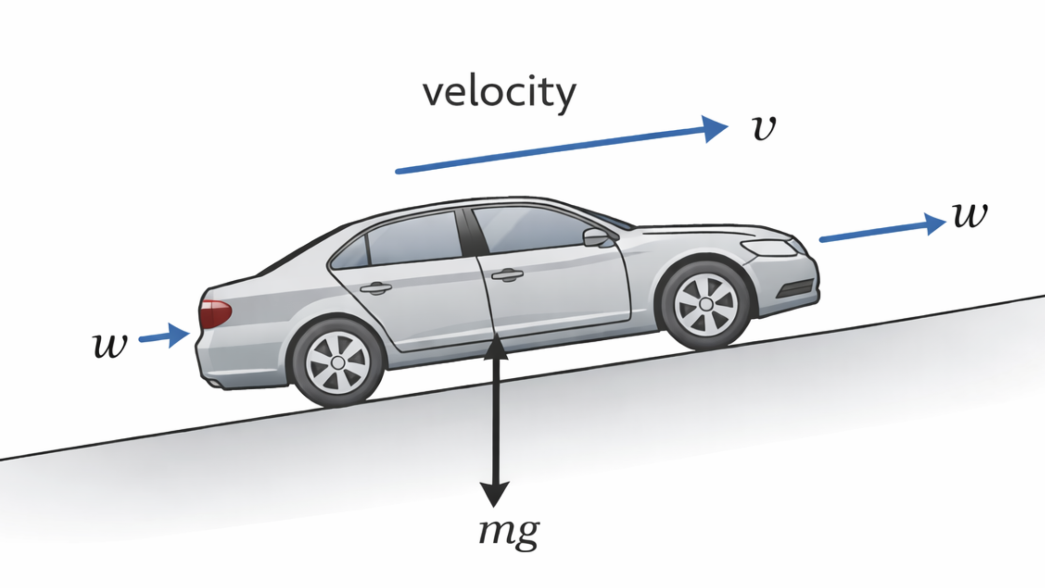
The change in the speed of a car with respect to time can be represented as the first-order, linear ODE

\[\dot{v}(t) = -\frac{1}{\tau} v(t) + \frac{K}{\tau} w(t) + d(t),\]

where \(v(t)\) is the speed at time \(t\), \(w(t)\) is the throttle command at time \(t\) (this will play the role of a control input), and the signal \(d\) represents the effects of disturbances (e.g., slope or wind). The constant parameters \(\tau\) and \(K\) capture the physical properties of the vehicle (e.g., mapping throttle to drive force) and the interaction of the vehicle with the environment (e.g., drag and rolling resistance).

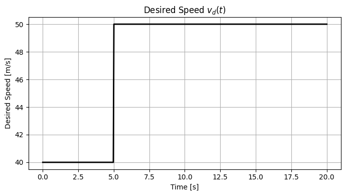
For a cruise control system, a common objective is making the difference between a driver-specified desired speed, call it \(v_d(t)\), and the actual speed \(v(t)\) small. Let us introduce a new signal, which we will refer to as the error denoted as \(e\):

\[e(t) = v_d(t) -v(t).\]

For a constant desired speed, \(\dot{v}_d(t) = 0\) for all \(t\geq 0.\) Then, \(\dot{e}(t) = -\dot{v}(t)\) and we can derive the following differential equation.

\[\dot{e}(t) = -\frac{1}{\tau} e(t) - \frac{K}{\tau} w(t) - d(t) +\frac{1}{\tau} v_d(t).\]

Our (control) objective will then be keeping \(|e(t)|\) as close to zero as possible.

The ODE for \(e\) includes three inputs: \(u,\) \(d\), and \(v_d\). While we will later work with multiple inputs, for now, let us consider that a control input has already been designed in the form of \(w(t) = k_p e(t)\) and there is no disturbance (i.e., \(d \equiv 0\)). Then, the model boils down to

\[\dot{e}(t) = -\left(\frac{1}{\tau}+ \frac{Kk_p}{\tau}\right) e(t) + \frac{1}{\tau} v_d(t).\]

This model will inform us about the changes in \(e\) with respect to \(v_d\).

By choosing \(x = e\), \(u=w\),

\[ A = -\left(\frac{1}{\tau}+ \frac{Kk_p}{\tau}\right) \text{, and } B = \frac{1}{\tau},\]

this ODE can be written in the form of the generic first-order system above.

What can we do with a model of a system?

1. Predict system behavior by solving the ODE (for some given initial condition and input).

2. Analyze the system behavior (for all initial conditions and inputs).

3. Design a controller to influence the system behavior.

While this class focuses on analysis of systems and design of controllers, simulation the system behavior (for some initial controls and/or inputs) offer visual insights. So, let’s start by simulating the cruise control model.

Simulating the system behavior

Let us pick some arbitrary values for \(A,\) \(B,\) \(v_d\) and initial conditions and simulate the system behavior.

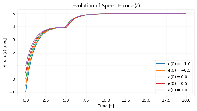
We will frequently simulate the behavior of the systems we work with, but, let us now go back to our main goal: analysis of system behavior and, eventually, design of controller so that the system we control behaves as we want it to behave.

What does it mean to be a solution to an ODE?

In a nutshell, a solution for an ODE satisfies “the ODE and its initial condition.” That is, if \(\bar{x}\) is a solution for the input signal \(u\), then

\[ \frac{d\bar{x}(t)}{dt} = A \bar{x}(t) + B u(t) \]

and

\[\bar{x}(0) = x_0.\]

Solution of the ODE for a first-order system

The solution is

\[ x(t) = e^{A t} x_0 + \int_{0}^{t} e^{A (t - \tau)} B\,u(\tau)\,d\tau. \]

We refer to “the solution” here rather than “a solution.” You may wonder whether there is always a solution to an ODE and, when it exists, it is unique.

How do we know that the above (candidate) solution is indeed a solution? Well, check whether it satisfies the conditions for being a solution.

Check the initial condition:

\[ x(0) = e^{A \cdot 0} x_0 + 0 = x_0. ~~✅ \]

Check whether it satisfies the differential equation:

\[\begin{split} \begin{aligned} \frac{d x(t)}{d t} &= A e^{A t} x_0 + A \int_{0}^{t} e^{A (t - \tau)} B\,u(\tau)\,d\tau + e^{A (t - t)} B\,u(t) - 0 \\[6pt] &= A \left[e^{A t} x_0 + \int_{0}^{t} e^{A (t - \tau)} B\,u(\tau)\,d\tau \right] + B\,u(t) \\[6pt] &= A\,x(t) + B \,u(t). ~~✅ \\[12pt] \end{aligned} \end{split}\]

How did we take the derivative of an integral? Recall: Leibniz integral rule

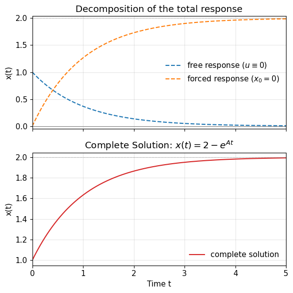
Complete solution = free response + forced response

Let us take a closer look at the solution:

\[ x(t) = \color{red}{e^{A t} x_0} + \color{blue} {\int_{0}^{t} e^{A (t - \tau)} B\,u(\tau)\,d\tau}. \]

The so-called free response is

\[ \color{red}{x_{free}(t) = e^{A t} x_0},\]

and it does not involve any contribution from input \(u\). It is therefore sometimes also called the unforced response.

The so-called forced response is

\[ \color{blue}{x_{forced}(t) = \int_{0}^{t} e^{A (t - \tau)} B\,u(\tau)\,d\tau},\]

and it does not involve any contribution from the initial condition and is solely driven by the input.

We can therefore analyze the free response and forced response separately to reason about the complete solution.

Free response and stability of a system

The free response (also called the natural response) is the part of the system’s output that arises solely from its initial conditions, with no external input applied.

Note that the only system parameter that appears in \(e^{At}x_0\) is \(A.\) Let’s analyze the free response for three cases with respect to the value of \(A.\)

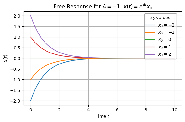
Case 1: \(A < 0\)

\[ x_{free}(t) = e^{A t} x_0 \to 0 \quad \text{as } t \to \infty \]

regardless of the value of \(x_0\). We will call the system (asymptotically) stable in this case. The free response converges to \(0\) for all initial conditions.

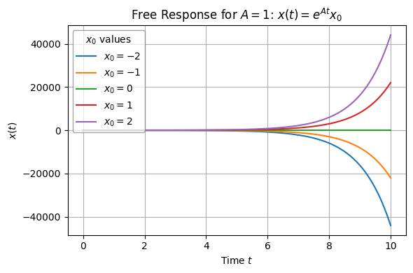
Case 2: \(A > 0\)

\[ |e^{A t} x_0| \text{ grows as } t \text{ increases unboundedly} \text{ (assuming $x_0 \neq 0$)} \]

We will call the system unstable in this case. The free response diverges for some initial conditions.

(For \(x_0 = 0\), \(x(t)\) remains at \(0\).)

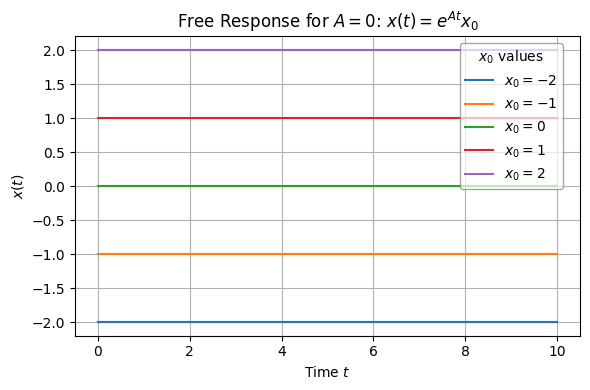
Case 3: \(A = 0\)

\[ x(t) = x_0 \text{ (constant over time)} \]

We call the system marginally stable in this case.

Let us now simulate the free response of a linear system for several different values of \(A\) and different initial conditions \(x_0.\)

Free response and time constant

Focus on the case \(A < 0\) (i.e., the system is asymptotically stable).

The time constant \(T\) of the system is defined as

\[ T = \frac{1}{|A|} = -\frac{1}{A}. \]

Hence,

\[ x(t) = e^{A t} x_0 = e^{-t/T} x_0. \]

Moral of the story: How much the gap from the system state \(x(t)\) is not merely a function of the initial condition and the time that has passed but it is a function of the ratio \(t/T\), i.e., how many time constants amount of time have passed.

Here is more on the practical uses of time constants: Time constants uses

Let’s look at an example.

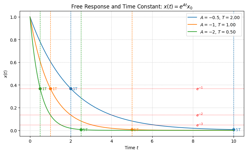
You may want to pause here and ask yourself how to interpret the figure above. You may also go into the code and change the system parameters and analyze how such changes affect the speed of response.

Forced response

Recall that the forced response for a first-order system is

\[ x_{forced}(t) = e^{A t} x_0 + \int_{0}^{t} e^{A (t - \tau)} B\,u(\tau)\,d\tau. \]

It determines how the system reacts to external inputs.

The table below summarizes a comparison between the free response and forced response of a stable system.

\[\begin{split} \boxed{ \begin{array}{l|l|c|c|l} \text{Part} & \text{Caused by} & \text{Exists if input = 0?} & \text{Depends on IC?} & \text{Behavior (for stable systems)} \\ \hline \textbf{Free response} & \text{The system’s own dynamics} & \text{Yes} & \text{Yes} & \text{Decays over time} \\ \textbf{Forced response} & \text{The external input} & \text{No} & \text{No} & \text{May persist as long as input acts} \end{array} } \end{split}\]

The forced response is determined by the input. Therefore, for a better understanding, we will look into several (canonical) input types.

Forced response with a step input (and zero initial conditions)

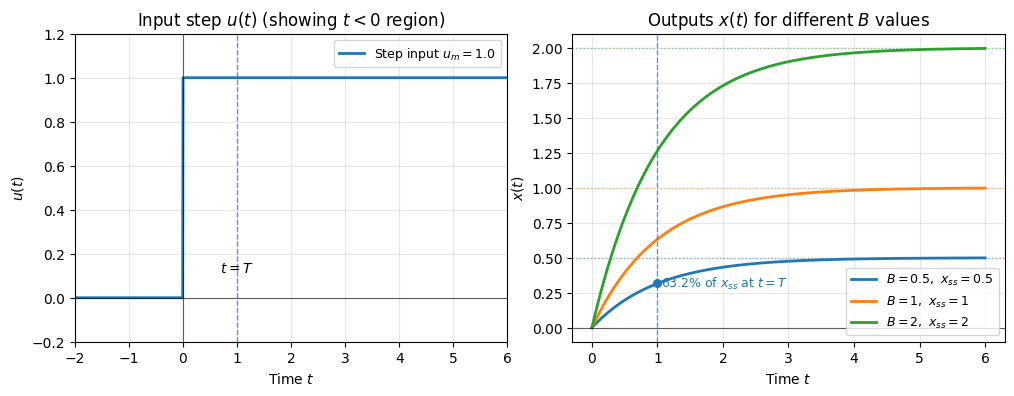
Consider the step input with magnitude \(u_m\):

\[\begin{split} u(t) = \begin{cases} 0, & t<0,\\[3pt] u_m, & t\ge 0. \end{cases} \end{split}\]

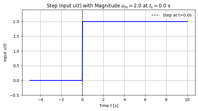
For this step input, the forced response becomes

\[\begin{split} \begin{aligned} x_{forced}(t) &= \int_{0}^{t} e^{A (t - \tau)} B\,u(\tau)\,d\tau \\ &= B\,u_m\, e^{A t} \int_{0}^{t} e^{-A\tau}\, d\tau \\ &= B\,u_m\, e^{A t}\,\frac{1 - e^{-A t}}{A} ~~~~~~(\text{assuming } A \neq 0)\\[2mm] &= \frac{B\,u_m}{A}\,(e^{A t} - 1). \end{aligned} \end{split}\]

Then, for a stable first-order system (i.e., A < 0), \(e^{At}\) approaches zero and \(x_{forced}\) approaches a so-called steady-state value as the \(t\) grows:

\[ x_{ss} = -\frac{B}{A}\,u_m, \]

and the steady-state gain (from the input to the state) for the system under step input is

\[\frac{x_{ss}}{u_m} = -\frac{B}{A}.\]

Similar expressions can be obtained for the output:

\[y_{ss} = \left( D-\frac{CB}{A}\right) u_m\]

and the steady-state gain from the step input to the system output s

\[\frac{y_{ss}}{u_m} = D-\frac{CB}{A}.\]

The forced response approaches its steady-state exponentially:

\[ x(t) = x_{ss}\,\big(1 - e^{A t}\big). \]

Recall the time constant is

\[ T = \frac{1}{|A|}. \]

At \(t = \tau\), the state reaches about 63.2% of its final value:

\[\begin{split} \begin{aligned} x(T) &= x_{ss}\,(1 - e^{-1}) \approx 0.632\,x_{ss} \\ x(2T) &= x_{ss}\,(1 - e^{-2}) \approx 0.869\,x_{ss}\\ x(3T) &= x_{ss}\,(1 - e^{-3}) \approx 0.950\,x_{ss}.\\ \end{aligned} \end{split}\]

Complete solution = free response + forced response (under step inputs).

The complete solution for a step input with magnitude \(u_m\) (applied at \(t=0\)) and an initial condition \(x_0\) is

\[ x(t) = x_0 e^{A t} - \frac{B}{A} u_m \left( 1 - e^{A t} \right) \]

and

\[ y(t) = Cx_0 e^{A t} - \frac{CB}{A} u_m \left( 1 - e^{A t} \right) + Du_m. \]

Let us look at an example.

Revisit the cruise control example

The code and the resulting figures below demonstrate the effect of the variables time constants and stead-state gains on the system response.

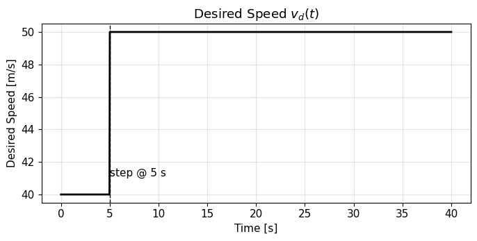
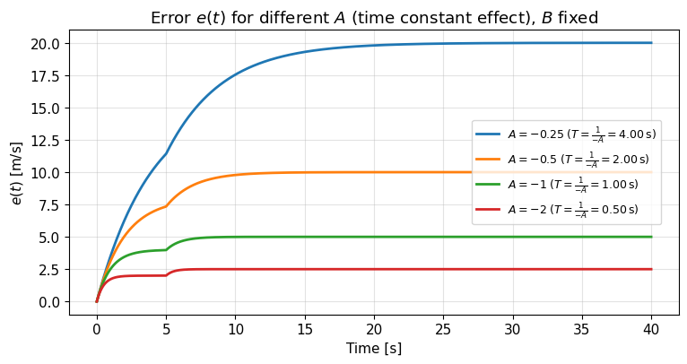
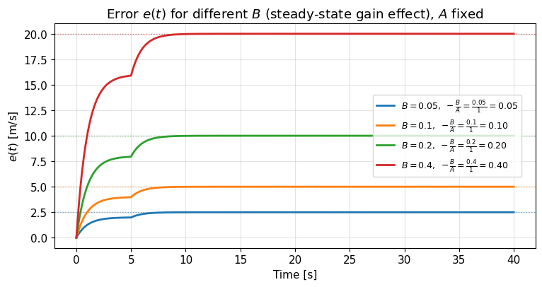
You may want to take some time to interpret the figures. Here are some guiding questions: (i) What value does the response settle toward? (ii) How fast does it do that and what determines the speed?

Response under sinusoidal inputs

Next, we will derive the response of a first-order linear system under sinusoidal inputs. We will derive this response through a seemingly unintuive way for convenience. We will derive the response first for complex-valued input signal of the following form:

\[ u(t) = \bar{u} e^{j \omega t}, \quad \text{for } t \ge 0,\]

where \(\bar{u}\) is a fixed, complex number, \(\omega\) is a fixed, real number, and \(j\) is the imaginary unit, i.e., \(j = \sqrt{-1}\).

Facts about complex numbers

Why are we interested in this complex-valued signal of time? Because it is directly related to (real-valued) sinusoidal signals (and it is easy to work with). To see the relation, let’s recall the Euler’s formula:

\[ e^{j \theta} = \cos(\theta) + j \sin(\theta) \]

for any real-valued \(\theta.\) Accordingly, the following holds:

\[ Real \left(e^{j \theta}\right) = cos (\theta) \text{ and } Imaginary \left(e^{j \theta}\right) = sin (\theta). \]

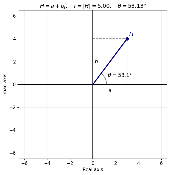
Recall that every complex number can be written in its polar form and its Cartesian form.

Cartesian form: \(H = a + j b\) where \(Real(H) = a\) and \(Imaginary(H) = b.\)

Polar form: \( H = r e^{j\theta}\) where \(r\) is the length and and \(\theta\) is the angle.

Here is an example plotted for \(H = 3 + 4j = 5 e^{j 0.93}\) (note: \(0.93 \text{ radians } \approx 53.13^o\)).

Saved plot as H_complex_plot.png

You can also play with the demo below to convince yourself that one can go back and forth between the two representations of complex numbers.

[Info] GUI unavailable (no display name and no $DISPLAY environment variable). Switching to CLI mode.\n

Complex Number Converter — Cartesian ↔ Polar
--------------------------------------------
Running in CLI mode (no GUI display detected).
Choose input form:
  [C] Cartesian (a + bj)
  [P] Polar (r, θ)
Your choice (C/P): C
Real part a: 3
Imag part b: 2

Polar form:
  r   = 3.605551
  θ   = 0.588003 rad  (33.690068°)

The relation between complex-valued exponential signals and real-valued sinusoidal signals

Let us now focus on the case where \(\theta = \omega t\) for \(\omega\) is a fixed, real number and \(t\) denotes an indeterminate variable (e.g., the time in our case).

Then, the Euler formula takes the form:

\[e^{j \omega t} = \cos(\omega t) + j \sin(\omega t).\]

Recall another fact: \(|e^{j \omega t}|=1\) for every \(\omega\) and \(t\), i.e., on the complex plane \(e^{j \omega t}\) is on the unit circle. The following animation shows how this point moves on the unit circle and how its real and imaginary parts map to sinusoidal signals of time.

This script is for fixed \(\omega\). Experiment with different values of \(\omega\) in the script and check its impact. Can you see why we will refer to \(\omega\) as “frequency”?

Once Loop Reflect

Response of \(\dot{x}(t) = A x + B u\) with \(u(t) = \bar{u} e^{j \omega t}\) and initial condition \(x(0) = x_0\).

Assumption: \(A < 0\) (i.e., the system is stable).

The general solution is given by

\[ x(t) = e^{A t} x_0 + \int_0^t e^{A (t - \tau)} B\, u(\tau) \, d\tau. \]

Substitute \(u(\tau) = \bar{u} e^{j \omega \tau}\):

\[ x(t) = e^{A t} x_0 + e^{A t} B \bar{u} \int_0^t e^{-A \tau} e^{j \omega \tau} d\tau \]

\[ x(t) = e^{A t} x_0 + e^{A t} B \bar{u} \int_0^t e^{(j \omega - A)\tau} d\tau. \]

Note that \(j\omega - A \neq 0\) since \(j \omega\) is imaginary and \(-A\) is real. Using this and taking the definite integral, we get

\[ x(t) = e^{A t} x_0 + \frac{B e^{A t}}{j \omega - A} \bar{u} \left[ e^{(j \omega - A)\tau} \right]_{\tau = 0}^{\tau = t} \]

\[ x(t) = e^{A t} x_0 + \frac{B e^{A t}}{j \omega - A} \bar{u} \left( e^{(j \omega - A)t} - 1 \right). \]

Simplify:

\[ x(t) = e^{A t} \left( x_0 - \frac{B \bar{u}}{j \omega - A} \right) + \frac{B }{j \omega - A} \bar{u} e^{j \omega t}. \]

If the output equation is \(y = Cx + D u\), then the output is

\[ y(t) = C e^{A t} \left( x_0 - \frac{B \bar{u}}{j \omega - A} \right) + \frac{C B}{j \omega - A} \bar{u} e^{j \omega t} + D \bar{u} e^{j \omega t}. \]

Steady-state response with input \(u(t) = \bar{u} e^{j \omega t}\).

Rearranging the terms in the above expression for \(y(t)\):

\[ y(t) = C e^{A t} \left( x_0 - \frac{B \bar{u}}{j \omega - A} \right) + \left( D + \frac{C B}{j \omega - A} \right) \bar{u} e^{j \omega t}. \]

Note: Since \(A < 0\), \(e^{A t} \to 0\) as \(t \to \infty\).

Hence,

\[ C e^{A t} \left( x_0 - \frac{B \bar{u}}{j \omega - A} \right) \to 0 \quad \text{as } t \to \infty. \]

At steady state (i.e., when \(e^{A t}\) is “sufficiently small”),

\[ u(t) = \bar{u} e^{j \omega t} \quad \Longrightarrow \quad y_{ss}(t) = \left( D + \frac{C B}{j \omega - A} \right) \bar{u} e^{j \omega t} \]

where \(y_{ss}(t)\) is the steady-state output.

We can then derive a central concept: the frequency response function:

\[ G(j \omega) = D + \frac{C B}{j \omega - A}. \]

What does all this say about real-valued (sinusoidal) inputs?

Answer: The real (imaginary) part of the output is the output corresponding to the real (imaginary) part of the input.

Reasoning: Let the system be given by

\[ \dot{x}(t) = \frac{dx(t)}{dt} = A x + B u \]

\[ y = C x + D u. \]

Write the complex-valued input, state, and output as

\[ u = u_r + j u_i, \quad x = x_r + j x_i, \quad y = y_r + j y_i. \]

Then,

\[ \frac{d x_r}{d t} + j \frac{d x_i}{d t} = A (x_r + j x_i) + B (u_r + j u_i) \]

\[ y_r + j y_i = C (x_r + j x_i) + D (u_r + j u_i). \]

The real and imaginary parts of these equations must hold individually:

\[ \dot{x}_r = A x_r + B u_r, \quad y_r = C x_r + D u_r \]

and

\[ \dot{x}_i = A x_i + B u_i, \quad y_i = C x_i + D u_i. \]

Consequently, the system responds independently to the real and imaginary parts of the input. That is, the real part of the output “corresponds” to the real part of the input, and the imaginary part of the output “corresponds” to the imaginary part of the input.

A few more facts (and observations) about complex numbers

Consider \(H \in \mathbb{C}\) (the set of complex numbers) with \(H \neq 0\).

The angle \(\angle H\) and the legth \(|H|\) of \(H\) satisfy

\[ \cos(\angle H) = \frac{\text{Re}(H)}{|H|}, \quad \sin(\angle H) = \frac{\text{Im}(H)}{|H|}. \]

It will be clear later why but, for now, let’s take a closer look at this complex number: \(H e^{j \theta}\), which is obtained by multiplying the complex number \(H\) and with \(e^{j \theta}.\) To this end, let us also write \(H\) in its Cartesian form \(H = H_R + j H_I\). Then,

\[ \text{Re}(H e^{j \theta}) = \text{Re}\!\left[ (H_R + j H_I)(\cos \theta + j \sin \theta) \right]. \]

Expanding:

\[ = H_R \cos \theta - H_I \sin \theta. \]

Express \(H_R\) and \(H_I\) in terms of \(|H|\) and \(\angle H\):

\[ H_R = |H| \cos(\angle H), \quad H_I = |H| \sin(\angle H). \]

Then,

\[ \text{Re}(H e^{j \theta}) = |H| \left( \cos(\angle H) \cos \theta - \sin(\angle H) \sin \theta \right). \]

Using the trigonometric identity for \(\cos(a + b)\):

\[ \text{Re}(H e^{j \theta}) = |H| \cos(\theta + \angle H). \]

Similarly,

\[ \text{Im}(H e^{j \theta}) = |H| \sin(\theta + \angle H). \]

Hence,

\[\begin{split}\begin{aligned} \text{Re}(H e^{j \theta}) &= |H| \cos(\theta + \angle H) \\ \text{Im}(H e^{j \theta}) &= |H| \sin(\theta + \angle H). \end{aligned} \end{split}\]

Constructing the sinusoidal steady-state output

The facts we already derived:

• For an exponential input

\[ u(t) = \bar{u} e^{j \omega t} \quad \Longrightarrow \quad y_{ss}(t) = G(j \omega) \bar{u} e^{j \omega t}, \]

where the output \(G(j \omega) \bar{u}\) of the frequency response function is, in general, a complex-valued quantity.

• For a complex number \(H\) and a real number \(\theta\) (for \(H \neq 0\)):

\[ \text{Re}(H e^{j \theta}) = |H| \cos(\theta + \angle H). \]

Now, consider a real-valued sinusoidal inputs with frequency \(\omega\). If

\[ u(t) = \cos(\omega t) = \text{Re}(e^{j \omega t}), \]

then

\[ y_{ss}(t) = |G(j \omega)| \cos(\omega t + \angle G(j \omega)). \]

If

\[ u(t) = \sin(\omega t) = \text{Im}(e^{j \omega t}), \]

then

\[ y_{ss}(t) = |G(j \omega)| \sin(\omega t + \angle G(j \omega)). \]

\(|G(j \omega)|\) is then called the steady-state gain of the system from sinusoidal inputs with frequency \(\omega\) to the output.

A special case boils down to the steady-state response under step inputs: If the input is constant, i.e.

\[ u(t) = 1 = e^{j \cdot 0 \cdot t}, \]

then

\[ y_{ss}(t) = |G(0)| = D - \frac{C B}{A}, \]

where recall that

\[|G(0)| = D - \frac{C B}{A}\]

is the steady-state gain of the system for step inputs.

If the inputs have a non-unit magnitude, the same results hold with the output scaled accordingly. Scaling the inputs, of course, does not impact the steady-state gains from the inputs to the outputs (assuming zero initial conditions).

Let’s put the results together (here \(u_m\) is a real constant):

\[\begin{split} \boxed{ \begin{array}{l|l} \textbf{Input} & \textbf{Steady-State Output} \\ \hline u_m \sin(\omega t) & u_m\,|G(j\omega)|\,\sin(\omega t + \angle G(j\omega)) \\ u_m \cos(\omega t) & u_m\,|G(j\omega)|\,\cos(\omega t + \angle G(j\omega)) \\ u_m & u_m\,|G(0)| \end{array} } \end{split}\]

We can derive several important observations:

• For a sinusoidal input, the steady-state output is also sinusoidal with the same frequency \(\omega\).

• The system does not change the frequency of the input — only its amplitude and phase.

\[ \text{Output frequency} = \text{Input frequency} = \omega. \]

• The output amplitude is scaled by the magnitude of the frequency response function \(|G(j\omega)|\):

\[ \text{Amplitude of output} = \alpha |G(j\omega)|. \]

• The system introduces a phase shift ( \angle G(j\omega) ) between the input and output:

\[ \text{Phase lag} = \angle G(j\omega). \]

• For a constant input \(u_m\):

\[ \text{Steady-state output} = u_m |G(0)|. \]

Overall, the frequency response function \(G(j \omega)\) plays a key role in the analysis of and design for first-order linear systems (and we will later see that these concepts generalize straightforwardly for linear systems).

Let’s take a look at an example.

\[\begin{split} \frac{dx(t)}{dt} = -x(t) + u(t) \\ y(t) = 2x(t). \end{split}\]

This corresponds to \(A=-1\), \(B=1\), \(C=2\), \(D=0\).

Is the system stable? Why?

The frequency response function is

\[ G(j\omega) = \frac{2}{j\omega + 1}. \]

We can use it to predict the steady-state output for any sinusoidal input. In particular let’s pick \(u(t) = sin(3t)\), i.e., \(\omega = 3\).

\[ G(j3) = \frac{2}{3j + 1} \]

\[ |G(j3)| = \frac{2}{|3j + 1|} = \frac{2}{\sqrt{10}} \approx 0.63 \]

\[ \angle G(j3) = \angle \frac{2}{3j + 1}. = 0 - \angle (3j + 1) \approx -1.25~\text{rad}. \]

Hence, the steady-state output is

\[ y_{\text{ss}}(t) \approx 0.63 \sin(3t - 1.25). \]

As predicted, the steady-state output is another sinusoidal signal with the same freqeuncy as the output. From the expression above, can you determine whether the peaks of the steady-state output will occur earlier or later than the peaks of the input signal?

A eigenvalues: [-1.]
Stable: True

Plot the frequency response function: Bode plots

The input to the frequency response function is a real-valued frequency value (e.g., the frequency of the input signal) and its output is complex-valued. Often, we use two plots to visualize this function: One for magnitude-vs-frequency and one for angle-vs-frequency. Such plots are also called Bode plots. (The angle is often also called the phase.)

/usr/local/lib/python3.12/dist-packages/scipy/signal/_filter_design.py:1230: BadCoefficients: Badly conditioned filter coefficients (numerator): the results may be meaningless
  b, a = normalize(b, a)

|G(j3)|  numeric = 0.632466,  analytic = 0.632456
∠G(j3)  numeric = -71.5647°,  analytic = -71.5651°

Control design for first-order systems

Let us consider a standard feedback interconnection.

The objective of control design to pick the controller so that the closed-loop system attains desired properties. This is a loaded sentence. We need to unpack it.

First, what is a closed-loop system?

At a high-level, a closed-loop control system uses measurements of the output (in addition to all other information that would be available to an open-loop system, see below) to adjust the control input, reducing the difference between the desired and actual output. (An example is a thermostat-controlled heating system that measures room temperature and adjusts heater power to reach the desired setpoint.)

It is worth contrasting a closed-loop system to an open-loop system. An open-loop control system operates without using feedback. The control action is based solely on the input command and the known system model.

How do we determine a closed-loop system?

In a standard feedback control system, we obtain the closed-loop system by mathematically combining the controller, plant, and feedback path. In other words, substitute all internal signals (e.g., the control signal) in terms of the state and external inputs. Let us work through an example.

Plant model (also referred to as open-loop model):

\[\begin{split} \begin{align} \dot{x} &= A x + B_1 u + B_2 d\\ y &= C x, \end{align} \end{split}\]

where \(x\) is the state, \(u\) is the control input, and \(d\) is the disturbance.

The control signal, for the sake of this example, is determined in the following form:

\[ u = K(r-y), \]

where \(K\) is a (controller) parameter to be determined and \(r\) is a reference input.

Note that the external inputs to this system are \(r\) and \(d\). And, also no that the control signal \(u\) is not an external input (or output). The external output is \(y\). Therefore, the closed-loop system will be in terms of \(x\), \(r\), and \(d\) with the output \(y\) and not \(u\).

We obtain the closed-loop model by plugging the control signal into the plant model:

\[\begin{split} \begin{align} \dot{x} &= A x + B_1 K (r - y) + B_2 d\\ y &= C x. \end{align} \end{split}\]

By substituting \(y = Cx\) in the state equation and rearranging, we obtain the closed-loop model

\[\begin{split} \begin{align} \dot{x} &= (A-B_1KC) x + B_1 K r + B_2 d\\ y &= C x. \end{align} \end{split}\]

Compare the closed-loop model to the open-loop model. What differences do you see?

Derive the closed-loop model for different control signals, e.g., \(u = K_1 r + K_2 y\).

Next, what may be some examples of the desired properties of a closed-loop system?

• The closed-loop system is stable.

• The closed-loop system has a time constant smaller that a given threshold. (Why smaller?)

• The steady-state gain from a specified input (e.g., \(r\) or \(d\) above) to a specified output (e.g., \(y\)) is smaller than, larger than, or equal to a specified value.

  • When do we care about “smaller” or “larger”?

  • Under what inputs, step or sinusoidal?

Example 1: A first-order model of cruise control

Consider the block diagram below for a cruise control system.

Goal: make the tracking error \(e = v - v_d\) small, where \(v_d\) denotes the desired velocity and \(v\) is the actual velocity.

The system dynamics are

\[ m \dot{v} + c v = F - m g \theta, \]

where \(v\) is the velocity, \(F\) is the control input (e.g., engine force) and \(\theta\) is the slope of the road (which acts as a disturbance).

We are interested in how the tracking error \(e = v - v_d\) evolves.

Starting with

\[ m \dot{v} + c v = F - m g \theta \]

and multiplying both sides by \(m\) gives

\[ m \dot{e} = m \dot{v}. \]

Then substitute the expression for \(\dot{v}\), we obtain

\[ m \dot{e} = -c v + F - m g \theta. \]

Since \(v = e + v_d\), we get

\[ m \dot{e} = -c(e + v_d) + F - m g \theta. \]

Simplify to

\[ m \dot{e} = -c e + F - c v_d - m g \theta. \]

Divide both sides by \(m\) to obtain

\[ \dot{e} = -\frac{c}{m} e + \frac{F - c v_d}{m} - g \theta. \]

In order to simplify the notation, we define a new variable

\[ u = \frac{F - c v_d}{m}, \]

which turns the error dynamics into

\[ \dot{e} = -\frac{c}{m} e + u - g \theta, \]

where \(u\) acts as the control input and \(g \theta\) acts as the disturbance term.

Let’s use a proportional control law

\[ u = k e. \]

Now, what should our design objective be?

Pick \(k\) such that:

• the closed-loop system is stable, and

• the steady-state error relative to a constant disturbance is small, e.g.

  \[ \left|\frac{e_{ss}}{\theta_{ss}}\right| \le 0.1. \]

The first step of control design is deriving the closed-loop dynamics (i.e., in this case, plug \(ke\) in for \(u\) in the open-loop dynamics for \(e\)):

\[ \dot{e} = \left(k - \frac{c}{m}\right)e - g \theta. \]

The system is stable if and only if

\[k - \frac{c}{m} < 0.\]

This is the condition to satisfy the first requirement.

At steady-state:

\[ e_{ss} = \frac{g \theta}{k - \frac{c}{m}}. \]

The steady-state gain from the disturbance to the tracking error is

\[ \frac{e_{ss}}{\theta_{ss}} = \frac{g}{k - \frac{c}{m}}. \]

We require

\[ \left| \frac{g}{k - \frac{c}{m}} \right| \le 0.1. \]

To satisfy both stability and steady-state requirements, one feasible choice is

\[ k = \frac{c}{m} - 10 g. \]

Example 2: Closed-loop response of a proportional controller

A plant with control input \(u\), disturbance input \(d\), internal state \(x\), and output \(y\), is governed by the equations

\[\begin{split}\begin{align*} \dot{x}(t) &= x(t) + d(t) + u(t)\\ y(t) &= x(t).\end{align*} \end{split}\]

A proportional controller is given by

\[ u(t) = -K y_m(t), \]

where \(y_m(t) = y(t) + n(t)\), and \(n\) represents additive measurement noise and \(K\) is a constant to be designed.

(a) Express the equations for the closed-loop interconnection (plant/controller/sensor) in the form

\[\begin{split} \begin{align*} \dot{x}(t) &= a x(t) + b_1 d(t) + b_2 n(t)\\ y(t) &= c_1 x(t) + d_{11} d(t) + d_{21} n(t)\\ u(t) &= c_2 x(t) + d_{21} d(t) + d_{22} n(t). \end{align*} \end{split}\]

Show answer

\[ \dot{x} = x+d-K(x+\eta)= (1 - K)x + d - K n, \]

\[ y = x, \]

\[ u = -Kx - Kn. \]

\[\begin{split} \boxed{ \begin{array}{c|c|c|c|c|c|c|c|c} a & b_1 & b_2 & c_1 & d_{11} & d_{21} & c_2 & d_{21} & d_{22} \\ \hline 1-K & 1 & -K & 1 & 0 & 0 & -K & 0 & -K \end{array} } \end{split}\]

(b) Under what condition (on \(K\)) is the closed-loop system stable?

Show answer

\[ 1 - K < 0 \]

(c) Assuming closed-loop stability, what is the steady-state gain (under step inputs) from \(d\) to \(y\)? (The answer will depend on \(K\).)

Show answer

\[ -\frac{1}{1-K} \]

(d) Assuming closed-loop stability, what is the steady-state gain (under step inputs) from \(d\) to \(u\)? (The answer will depend on \(K\).)

Show answer

\[ \frac{K}{1-K} \]

(e) Assuming closed-loop stability, what is the time constant of the closed-loop system? (The answer will depend on \(K\).)

Show answer

\[ -\frac{1}{1-K} \]

Example 3: Open-loop versus closed-loop control

Consider a first-order system \(P\), with inputs \((d,u)\) and output \(y\), governed by

\[\begin{split} \begin{align*} \dot{x}(t)&=a\,x(t)+b_1 d(t)+b_2 u(t)\\ y(t)&=c\,x(t). \end{align*} \end{split}\]

1. Open-loop gains:

Assume \(P\) is stable (i.e., \(a<0\)). For \(P\) itself, what is the steady-state gain from \(u\) to \(y\) (assuming \(d\!\equiv\!0\))? Call this gain \(G\). Moreover, what is the steady-state gain from \(d\) to \(y\) (assuming \(u\!\equiv\!0\))? Call this gain \(H\).

Show answer

\[ G=-\frac{b_2 c}{a},\qquad H=-\frac{b_1 c}{a}. \]

2. Proportional control and closed-loop model

\(P\) is controlled by a proportional controller of the form

\[ u(t)=K_1 r(t)+K_2[\,r(t)-(y(t)+n(t))\,]. \]

Here \(r\) is the reference (the desired value of \(y\)), \(n\) is measurement noise (so that \(y + n\) is the measurement of \(y\)), and \(K_1,K_2\) are controller gains.

By substituting for \(u\), write the state equation in the form

\[ \dot{x}(t)=A\,x(t)+B_1 r(t)+B_2 d(t)+B_3 n(t). \]

Moreover, express the output \(y\) and control input \(u\) as functions of \(x\) and the external inputs \((r, d, n)\) as

\[\begin{split} \begin{align*} y(t) &= C_1x(t) + D_{11}r(t) + D_{12}d(t) + D_{13}n(t)\\ u(t) &= C_2x(t) + D_{21}r(t) + D_{22}d(t) + D_{23}n(t). \end{align*} \end{split}\]

All of the symbols \((A,B_1, . . . ,D_{23})\) will be functions of the lower-case given symbols and the controller gains.

Show answer

We have

\[\begin{split} \begin{align*} \dot{x}&=ax+b_1d+b_2(K_1r+K_2r-K_2y-K_2n)\\ &=ax+b_1d+b_2(K_1+K_2)r-b_2K_2cx-b_2K_2n\\ &=(a-b_2K_2c)\,x+b_2(K_1+K_2)\,r+b_1d-b_2K_2n. \end{align*} \end{split}\]

\[\begin{split} \boxed{ \begin{array}{c|ccc} A & B_1 & B_2 & B_3\\ \hline a-b_2K_2c & b_2(K_1+K_2) & b_1 & -b_2K_2 \end{array} } \end{split}\]

\[\begin{split} \begin{align*} y&=cx,\\ u&=K_1r+K_2(r-cx-n) \\&=-K_2c\,x+(K_1+K_2)r-K_2n. \end{align*} \end{split}\]

\[\begin{split} \boxed{ \begin{array}{c|cccc} & C_1 & D_{11} & D_{12} & D_{13}\\ \hline y & c & 0 & 0 & 0 \end{array} } \qquad \boxed{ \begin{array}{c|cccc} & C_2 & D_{21} & D_{22} & D_{23}\\ \hline u & -K_2c & K_1+K_2 & 0 & -K_2 \end{array} } \end{split}\]

3. Closed-loop stability and steady-state gains

Under what conditions is the closed-loop system stable? What is the steady-state gain from \(r\) to \(y\) (assuming \(d=0\) and \(n=0\))? What is the steady-state gain from \(d\) to \(y\) (assuming \(r=0\) and \(n=0\))?

Show answer

\[ \text{Stability: } a-b_2K_2c<0, \]

\[ \text{Gain }r\!\to\!y=-\frac{b_2(K_1+K_2)c}{a-b_2K_2c}, \]

\[ \text{Gain }d\!\to\!y=-\frac{b_1c}{a-b_2K_2c}. \]

4. Design #1 (Open-loop / Feed-forward)

In this part, we design a feedback control system that actually had no feedback (\(K_2=0\)). The control system is called open-loop or feed-forward, and will be based on the steady-state gain \(G\) (from \(u\rightarrow y\)) of the plant. The open-loop controller is simple - simply invert the gain of the plant, and use that for \(K_1\). Hence, we pick

\[ K_1=\frac{1}{G} \]

and \(K_2=0\). Call this Design #1.

(a) For Design #1, compute the steady-state gains from each of \((r,d,n)\) to each of \((y,u)\).

Show answer

\[\begin{split} \boxed{ \begin{array}{c|ccc} & r & d & n\\ \hline y & -\frac{b_2cK_1}{a}=-\frac{b_2c}{a}\frac{1}{G}=1 & -\dfrac{b_1 c}{a} & -\frac{b_2K_2}{a-b_2K_2c}=0\\[6pt] u & K_1+K_2-\frac{-K_2cb_2(K_1+K_2)}{a-b_2K_2c}=K_1=\dfrac{1}{G} & -\frac{K_2cb_1}{a-b_2K_2c}=0 & -K_2-\frac{-K_2c(-b_2K_2)}{a-b_2K_2c}=0 \end{array} } \end{split}\]

(b) Comment on the steady-state gain from \(r\!\to\!y\).

Show answer

It equals 1 — perfect reference tracking since \(G\) was selected as the steady-state gain from \(u\) to \(y\).

(c) Comment on the relationship between the steady-state gain from \(d\!\to\!y\) without any control (i.e., H computed above) and the steady-state gain from \(d\!\to\!y\) as computed in a.

Show answer

Both \(-\dfrac{b_1 c}{a}\) — no improvement in disturbance rejection.

(d) Comment on the steady-state gain from \(d\) to \(u\) in Design #1. Based on \(d\)’s eventual effect on \(u\), is the answer in part c surprising?

Show answer

\[ \text{Gain}_{d\to u}=0 \]

This is because the control signal \(u\) does not depend on \(d\).

(e) Comment on the steady-state gain from \(n\) to both \(y\) and \(u\) in Design #1. Remember that Design #1 actually does not use feedback…

Show answer

\[ \text{Gain}_{n\to y}=0,\qquad \text{Gain}_{n\to u}=0 \]

Noise does not affect either output or control, because \(K_2=0\).

(f) What is the time-constant of the system with Design #1.

Show answer

\[ \tau=-\frac{1}{a-b_2K_2c}=-\frac{1}{a} \]

5. Design #2 (True feedback control)

Now design a true feedback control system. This is Design #2. Pick \(K_2\) so that the closed-loop steady-state gain from \(d\!\to\!y\) is at least 5 times less than the uncontrolled steady-state gain from \(d\!\to\!y\) (which we called H).

Show answer

The uncontroled gain is

\[-\frac{cb_1}{a}\]

while the closed-loop gain is

\[-\frac{b_1c}{a-b_2K_2c}.\]

Therefore,

\[ -\frac{b_1 c}{a-b_2K_2c}\le -\frac{1}{5}\frac{cb_1 }{a} \Rightarrow K_2\ge -\frac{4a}{b_2c}. \]

Constrain your choice of \(K_2\) so that the closed-loop system is stable.

Show answer

\[ a-b_2K_2c<0 \Longrightarrow K_2>\frac{a}{b_2c},\qquad \text{choose }K_2=-\frac{4a}{b_2c} \]

Since we are working fairly general, for simplicity, you may assume \(a<0\) and \(b_1>0\), \(b_2>0\) and \(c > 0\).

(a) With \(K_2\) chosen, pick \(K_1\) so that the closed-loop steady-state gain from \(r\!\to\!y\) is 1.

Show answer

\[ -\frac{b_2(K_1+K_2)c}{a-b_2K_2c}=1 \Rightarrow K_1=-\frac{a}{b_2c}. \]

(b) What is the time-constant of the closed-loop system?

Show answer

\[ \tau=-\frac{1}{a-b_2K_2c} =-\frac{1}{a-b_2c(-\frac{4a}{b_2c})} =-\frac{1}{5a}. \]

(c) What is the steady-state gain from \(d\!\to\!u\)? How does this compare to the previous case (feedforward)?

Show answer

\[ \text{Gain}_{d\to u}=-\frac{-K_2cb_1}{a-b_2K_2c} =-\frac{4}{5}\frac{b_1}{b_2}. \]

This means the disturbance now has an effect on the control signal.

(d) With \(K_2\ne0\), does the noise \(n\) now affect \(y\)? (Find the gain from \(n\) to \(y\). )

Show answer

\[ \text{Gain}_{n\to y}=-\frac{-b_2K_2c}{a-b_2K_2c}=-\frac{4}{5} \]

The noise now affects the output, which is the price we pay for feedback control.

Summary: Design #2 — steady-state gain tables

Show answer

\[\begin{split} \boxed{ \begin{array}{c|ccc} & r & d & n\\[3pt] \hline y & 1 & -\dfrac{b_1 c}{a-b_2K_2c} & \dfrac{b_2K_2c}{a-b_2K_2c}\\[10pt] u & K_1+K_2 & \dfrac{K_2cb_1}{a-b_2K_2c} & -K_2 \end{array} } \end{split}\]

With \(K_2=-\dfrac{4a}{b_2c}\) and \(K_1=-\dfrac{a}{b_2c}\):

\[\begin{split} \boxed{ \begin{array}{c|ccc} & r & d & n\\[3pt] \hline y & 1 & -\dfrac{1}{5}\dfrac{b_1 c}{a} & -\dfrac{4}{5}\\[10pt] u & -\dfrac{5a}{b_2c} & -\dfrac{4}{5}\dfrac{b_1}{b_2} & \dfrac{4a}{b_2c} \end{array} } \end{split}\]

Summary: Design #1 vs Design #2 — comparison table

Show answer

\[\begin{split} \boxed{ \begin{array}{l|cc} & \text{Design #1 (Open-loop)} & \text{Design #2 (Feedback)}\\ \hline K_1 & -\dfrac{a}{b_2c} & -\dfrac{a}{b_2c}\\[4pt] K_2 & 0 & -\dfrac{4a}{b_2c}\\[4pt] \text{Closed-loop pole }(A) & a & 5a\\[4pt] \text{Time constant }(\tau) & -\dfrac{1}{a} & -\dfrac{1}{5a}\\[4pt] \text{Gain }r\!\to\!y & 1 & 1\\[4pt] \text{Gain }d\!\to\!y & -\dfrac{b_1c}{a} & -\dfrac{1}{5}\dfrac{b_1c}{a}\\[4pt] \text{Gain }n\!\to\!y & 0 & -\dfrac{4}{5}\\[4pt] \text{Gain }d\!\to\!u & 0 & -\dfrac{4}{5}\dfrac{b_1}{b_2}\\[4pt] \text{Gain }n\!\to\!u & 0 & \dfrac{4a}{b_2c} \end{array} } \end{split}\]