![]()
All rights reserved. For enrolled students only. Redistribution prohibited.
Optimal Control#
Motivation
Linear quadratic regulator
Relation to pole placement
Examples
Motivation for optimal control#
Up to this point, we designed controllers so that the closed-loop system meets given explicit specifications, e.g.,
is stable,
has desired transient behavior,
tracks references,
rejects disturbances.
Our approach has been translating these specifications to contraints, e.g., on the roots of the closed-loop characteristic polynomial or, equivalent, the eigenvalues of the closed-loop “A” matrix. This approach works well, but it also raises a natural question: What if we do not know, for example, exactly what values for the roots of the closed-loop characteristic polynomial are “best,” but we do know what we care about qualitatively? Optimal control provides a different perspective on control design.
Rather than specifying controller parameters directly, optimal control starts by specifying what we want to optimize. Typical objectives include:
keeping the state small,
keeping the control effort small,
balancing performance against effort.
The controller is then chosen automatically to optimize these objectives, subject to the system dynamics.
The simplest optimal control problem: Linear Quadratic Regulator (LQR)#
Optimal control is a broad framework for designing controllers by minimizing a performance objective, subject to system dynamics. We focus on the simplest possible optimal control problem, the linear quadratic regulator (LQR).
The system dynamics are linear:
The performance objective in LQR is expressed through a cost function of the form
where
the positive semidefinite matrix \(Q\) penalizes deviations of the state from the origin, and
the positive definite matrix \(R\) penalizes the use of control effort.
The quadratic structure gives rise to several features:
it penalizes large deviations more heavily than small ones,
it leads to mathematically tractable solutions,
and it naturally expresses tradeoffs between competing objectives.
To build intuition for the LQR cost function, we examine how the cost accumulates along a single closed-loop trajectory.
The figures below show the response of a linear system under a fixed stabilizing state-feedback controller. Along with the state trajectory and control input, we explicitly plot the quantities that appear inside the LQR cost:
the instantaneous state penalty \(x(t)^\top Q x(t)\),
the instantaneous control penalty \(u(t)^\top R u(t)\),
and their sum, which forms the instantaneous cost integrand.
We also plot the cumulative integrals of these terms over time, illustrating how the total cost \(J\) is built up as the system evolves.
These plots highlight several important points:
the cost is accumulated continuously over time, not just at steady state,
large transients in either the state or the input contribute significantly to the total cost,
and the relative weighting of state deviations versus control effort determines which parts of the trajectory dominate the cost.
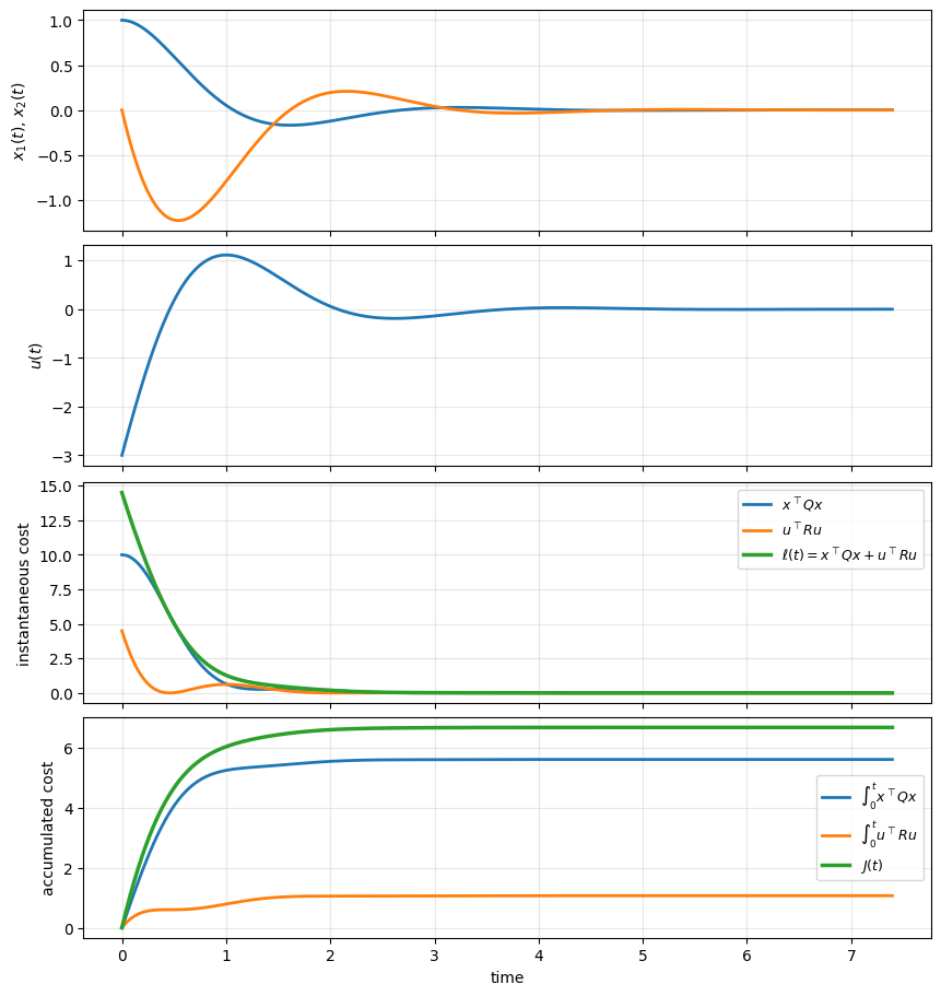
Final accumulated cost at t=7.39:
  integral of x^T Q x  = 5.6091
  integral of u^T R u  = 1.0674
  total J              = 6.6765
Example on the roles of the state and input parts of the costs#
To build intuition for the LQR cost function, we consider a simple two-dimensional linear system and compare controllers obtained from different choices of the weighting matrices \(Q\) and \(R\).
In all cases, the system dynamics and initial condition are the same. The only difference is how much we penalize state deviations versus control effort.
By emphasizing different terms in the cost, we obtain controllers that:
drive the state to the origin quickly using larger inputs,
use smaller control inputs but converge more slowly,
or balance these two objectives.
The figures below show how these design choices affect the state trajectories, the control input, and how the cost accumulates over time.
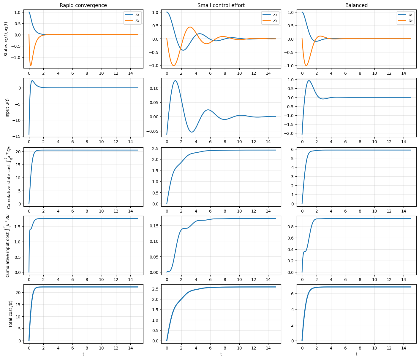
Gains and final costs:

Rapid convergence
K = [[14.452   8.4883]]
Final ∫ x^T Q x dt = 20.4899
Final ∫ u^T R u dt = 1.7605
Final J            = 22.2504

Small control effort
K = [[0.0616 0.1387]]
Final ∫ x^T Q x dt = 2.4098
Final ∫ u^T R u dt = 0.1723
Final J            = 2.5821

Balanced
K = [[2.062  1.7946]]
Final ∫ x^T Q x dt = 5.8837
Final ∫ u^T R u dt = 0.9378
Final J            = 6.8216
An interactive example: Exploring the \(Q\) and \(R\) trade-off#
Consider the second-order unstable plant
with initial condition \(x(0) = [1, 0]^\top\).
Let us use a cost function of the following form:
where \(q_1\), \(q_2\) and \(R\) are positive scalars.
Use the sliders to adjust \(q_1\), \(q_2\), and \(R\), and observe:
State trajectories: How quickly do the states converge to zero?
Control effort: How much actuator authority is required?
Accumulated cost: What is the total cost \(J\)?
Try these experiments:
Increase \(q_1\) while keeping \(q_2\) and \(R\) fixed. What happens to \(x_1(t)\)?
Increase \(R\) while keeping \(Q\) fixed. What happens to \(u(t)\) and the convergence speed?
Can you find settings that minimize the total cost \(J\)?
Note: Please use Colab for this experiment
plot_lqr
def plot_lqr(q1=10, q2=1, R=1)
<no docstring>
What does LQR produce?#
The solution to the LQR problem has the form
where the feedback gain \(K\) depends on the system matrices \(A,B\) and the chosen weights \(Q,R\).
Importantly:
the controller is linear,
the feedback gain is constant,
and the stability of the closed-loop system is guaranteed under mild conditions.
Thus, LQR fits naturally into the state-feedback framework we have already discussed. In pole placement, we specify where we want the eigenvalues of the closed-loop system matrix to be.
In LQR, we specify what we care about, e.g., how large the state is allowed to be and how expensive it is to apply control. The resulting closed-loop pole locations emerge as a consequence of the optimization, rather than being chosen explicitly.
The example below illustrated this relation.
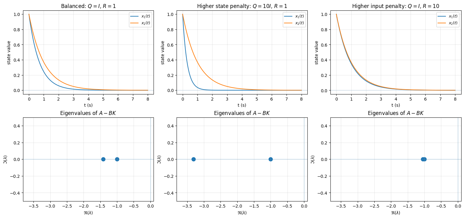
We design three LQR controllers for the same system (which is unstable) with different choices of the weighting matrices \(Q\) and \(R\). The three cases illustrate different design priorities:
Balanced state and input penalty: The matrices \(Q=I\) and \(R=1\) penalize state deviation and control effort equally. The resulting controller provides a reasonable compromise between convergence speed and input magnitude.
Higher state penalty: The choice \(Q=10I\), \(R=1\) places greater emphasis on keeping the state small. This typically leads to faster convergence, but at the cost of larger control inputs and more aggressive closed-loop dynamics.
Higher input penalty: The choice \(Q=I\), \(R=10\) places greater emphasis on limiting control effort. The controller uses smaller inputs, but the state converges more slowly.
The figure shows, for each case, the resulting state trajectories and the corresponding closed-loop eigenvalues of \(A-BK\). Comparing the columns illustrates how changing the relative weights in the cost function directly affects both the time-domain behavior and the location of the eigenvalues of the closed-loop system matrix.
Open-loop eigenvalues(A): [ 1. -1.]
Open-loop stable? False
Computing the LQR solution in practice#
A natural question is how the optimal feedback gain is actually computed.
The key theoretical result—whose derivation we do not cover here—is that the LQR problem can be solved by finding the solution of an algebraic Riccati equation (ARE). This equation can be solved efficiently using standard numerical algorithms, even for higher-order systems.
In practice, we rarely compute the Riccati solution by hand. Instead, we rely on well-tested routines available in standard control software.
In Python, LQR is implemented in the Python Control Systems Library (the control package) using the command
K, S, E = control.lqr(A, B, Q, R)
K: the optimal state-feedback gain, used as \(u(t)=-Kx(t)\).
S: the solution of the algebraic Riccati equation.
E: the eigenvalues of the closed-loop matrix \(A-BK\).
In MATLAB, the same computation is available through the Control System Toolbox using
[K,S,E] = lqr(A,B,Q,R)
How is the algebraic Riccati equation, and its solution \(S\), connected to LQR?
See here.
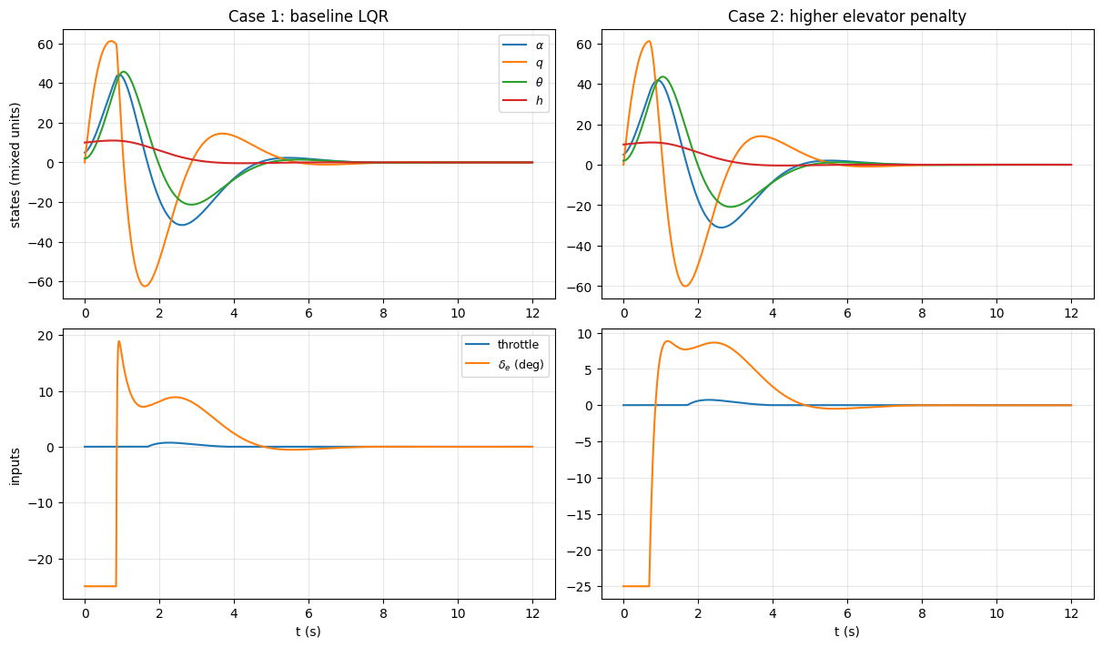
Aircraft LQR example#
We now consider a higher-order aircraft example to illustrate how LQR design choices influence closed-loop behavior in a realistic setting. The model is a linearized longitudinal dynamics model of an F-16 aircraft about a steady trim condition. The state vector includes variables associated with both fast and slow motion, such as angle of attack, pitch rate, pitch angle, and altitude, while the control inputs include throttle and elevator deflection.
The model is written in state-space form as
where the state and input are
Here:
\(V_a\) is airspeed deviation,
\(h\) is altitude deviation,
\(\alpha\) is angle of attack,
\(\theta\) is pitch angle,
\(q\) is pitch rate,
\(\text{power}\) is an engine/thrust-related state, and
\(\delta_e\) is elevator deflection.
The matrices \(A\) and \(B\) come from a standard small-perturbation linearization of the F-16 longitudinal dynamics at a specified trim condition (altitude, speed, configuration), as presented in Aircraft Control and Simulation: Dynamics, Controls Design, and Autonomous Systems, John Wiley & Sons, Inc., Hoboken, NJ, 2015.
Case 1: a reasonable design: In the first case, we choose weighting matrices \(Q\) and \(R\) that place comparable penalties on state deviations and control effort. This produces a stable closed-loop system with fast convergence and well-damped motion.
However, inspection of the control inputs reveals a potential issue: the elevator deflection can be large or highly active. While this behavior is optimal with respect to the chosen cost function, it may be undesirable from an engineering standpoint due to actuator limits, wear, or comfort.
Case 2: refining the design by adjusting the input penalty: In the second case, we keep the state weighting matrix \(Q\) unchanged and increase the penalty on the elevator input in \(R\).
This change reflects a revised design priority: we now value smoother and smaller elevator motions more strongly, even if that means accepting slightly slower or less aggressive state regulation.
Open-loop eigenvalues(A): [ 0.    +0.j     -0.8   +0.j     -0.8779+1.8577j -0.8779-1.8577j
  0.2425+0.j     -0.3066+0.j    ]

Closed-loop eigenvalues (Case 1): [-50.6299+0.j      -0.9425+1.2013j  -0.9425-1.2013j  -2.2678+0.j
  -1.5587+0.j      -0.3636+0.j    ]
Closed-loop eigenvalues (Case 2): [-4.2027+0.j     -0.9949+1.1664j -0.9949-1.1664j -2.2695+0.j
 -1.8624+0.j     -0.3633+0.j    ]